
Context-Aware Multi-Agent Coordination: Learning Correlated Equilibria Under Situational Constraints
Proceedings of the Thirty-Fifth International Joint Conference on Artificial Intelligence. Main Track. Pages 463-471.
https://doi.org/10.24963/ijcai.2026/53
Keywords
- Agent-based and Multi-agent Systems: Multi-agent learning
- Agent-based and Multi-agent Systems: Coordination and cooperation
Abstract
Effective multi-agent coordination requires aligning incentives while adhering to complex requirements. However, real-world systems often impose situational constraints, context-dependent requirements triggered only under specific conditions, which challenge standard Correlated Equilibria (CE) solutions. We propose Situational-Constrained Density-Based Correlated Equilibria (SC-DBCE), a novel concept in Markov Games that formalizes situational constraints as logic implications. To solve this, we introduce Situational-Constrained Correlated Policy Iteration (SC-CPI), a reinforcement learning algorithm employing a smooth Log-Sum-Exp mechanism for constraint optimization. Evaluations on multi-agent games, smart grids, and warehouse robotics demonstrate that SC-CPI consistently outperforms baselines in both equilibrium quality and constraint adherence. To our knowledge, this is the first method learning CE under situational constraints.
- [Altman and Shwartz, 2000] Eitan Altman and Adam Shwartz. Constrained markov games: Nash equilibria. In Advances in dynamic games and applications, pages 213-221. Springer, 2000.
- [Aumann, 1974] Robert J Aumann. Subjectivity and corre- lation in randomized strategies. Journal of mathematical Economics, 1(1):67-96, 1974.
- [Aumann, 1987] Robert J Aumann. Correlated equilibrium as an expression of bayesian rationality. Econometrica: Journal of the Econometric Society, pages 1-18, 1987.
- [Durfee et al., 1999] Edmund H Durfee, Charles L Ortiz Jr, Michael J Wolverton, et al. A survey of research in dis- tributed, continual planning. Ai magazine, 20(4):13-13, 1999.
- [Foerster et al., 2016] Jakob Foerster, Ioannis Alexandros Assael, Nando De Freitas, and Shimon Whiteson. Learn- ing to communicate with deep multi-agent reinforcement learning. Advances in neural information processing sys- tems, 29, 2016.
- [Garcıa and Fernández, 2015] Javier Garcıa and Fernando Fernández. A comprehensive survey on safe reinforce- ment learning. Journal of Machine Learning Research, 16(1):1437-1480, 2015.
- [González-Soto et al., 2025] Martín González-Soto, Manuel Fernández-Veiga, Rebeca P Díaz-Redondo, Bruno Fernández-Castro, and Ana Fernández-Vilas. Ic4net: Decentralized communication for continual multi-agent learning. IEEE Access, 13:199352-199365, 2025.
- [Greenwald et al., 2003] Amy Greenwald, Keith Hall, Roberto Serrano, et al. Correlated q-learning. In ICML, volume 3, pages 242-249, 2003.
- [Hallak et al., 2015] Assaf Hallak, Dotan Di Castro, and Shie Mannor. Contextual markov decision processes. arXiv preprint arXiv:1502.02259, 2015.
- [Han et al., 2007] Zhu Han, Charles Pandana, and KJ Ray Liu. Distributive opportunistic spectrum access for cogni- tive radio using correlated equilibrium and no-regret learn- ing. In 2007 IEEE wireless communications and network- ing conference, pages 11-15. IEEE, 2007.
- [Huang et al., 2022] Zijian Huang, Meng-Fen Chiang, and Wang-Chien Lee. Line: Logical query reasoning over hi- erarchical knowledge graphs. In Proceedings of the 28th ACM SIGKDD Conference on Knowledge Discovery and Data Mining, pages 615-625, 2022.
- [Littman, 1994] Michael L Littman. Markov games as a framework for multi-agent reinforcement learning. In Ma- chine learning proceedings 1994, pages 157-163. Else- vier, 1994.
- [Markowitz, 1952] Harry Markowitz. Portfolio selection*. The Journal of Finance, 7(1):77-91, 1952.
- [Ortiz et al., 2007] Luis E Ortiz, Robert E Schapire, and Sham M Kakade. Maximum entropy correlated equilib- ria. In Artificial Intelligence and Statistics, pages 347-354.
- PMLR, 2007.
- [Pu, 2021] Lida Pu. Fairness of the distribution of public medical and health resources. Frontiers in public health, 9:768728, 2021.
- [Qin et al., 2021] Zengyi Qin, Yuxiao Chen, and Chuchu Fan. Density constrained reinforcement learning. In Inter- national Conference on Machine Learning, pages 8682- 8692. PMLR, 2021.
- [Rantzer, 2001] Anders Rantzer. A dual to lyapunov's stabil- ity theorem. Systems & Control Letters, 42(3):161-168, 2001.
- Ren et al., ] Hongyu Ren, Weihua Hu, and Jure Leskovec. Query2box: Reasoning over knowledge graphs in vector space using box embeddings. In International Conference on Learning Representations.
- [Sessa et al., 2020] Pier Giuseppe Sessa, Ilija Bogunovic, Andreas Krause, and Maryam Kamgarpour. Contex- tual games: Multi-agent learning with side informa- tion. Advances in Neural Information Processing Systems, 33:21912-21922, 2020.
- [Sun et al., 2025] Lijun Sun, Yijun Yang, Qiqi Duan, Yuhui Shi, Chao Lyu, Yu-Cheng Chang, Chin-Teng Lin, and Yang Shen. Multi-agent coordination across diverse ap- plications: A survey. arXiv preprint arXiv:2502.14743, 2025.
- [Syed et al., 2008] Umar Syed, Michael Bowling, and Robert E Schapire. Apprenticeship learning using linear programming. In Proceedings of the 25th international conference on Machine learning, pages 1032-1039, 2008.
- Torreno et al., ] Alejandro Torreno, Eva Onaindia, and Os- car Sapena. Fmap: Distributed cooperative multi-agent planning. [Wurman et al., 2008]
- Peter R Wurman, Raffaello D'Andrea, and Mick Mountz. Coordinating hun- dreds of cooperative, autonomous vehicles in warehouses. AI magazine, 29(1):9-9, 2008.
- [Yu et al., 2014] Tao Yu, HZ Wang, Bin Zhou, Ka Wing Chan, and J Tang. Multi-agent correlated equilibrium q (λ) learning for coordinated smart generation control of interconnected power grids. IEEE transactions on power systems, 30(4):1669-1679, 2014.
- [Zhang et al., 2023] Libo Zhang, Yang Chen, Toru Takisaka, Bakh Khoussainov, Michael Witbrock, and Jiamou Liu. Learning density-based correlated equilibria for markov games. In Proceedings of the 2023 International Con- ference on Autonomous Agents and Multiagent Systems, pages 652-660, 2023.
- [Zhang et al., 2024] Libo Zhang, Yuly Wu, Weidong Li, Song Yang, Yang Chen, Kaiqi Zhao, and Jiamou Liu. Op- timizing resource distribution towards energy justice in resilient smart grids. In Principle and Practice of Data and Knowledge Acquisition Workshop, pages 236-245. Springer, 2024.
- [Zhang et al., 2025] Libo Zhang, Yang Chen, Toru Takisaka, Kaiqi Zhao, Weidong Li, and Jiamou Liu. Situational- constrained sequential resources allocation via reinforce- ment learning. In Proceedings of the Thirty-Fourth Inter- national Joint Conference on Artificial Intelligence, IJCAI '25, 2025.
References were extracted automatically from the PDF and may contain errors.
Full text extracted automatically from the PDF; figures, tables and equations may differ. The PDF is the version of record.
1 Introduction
Multi-Agent coordination is the problem of designing strategies that align agents toward a collective objective while respecting individual interests [Sun et al., 2025]. This challenge is prevalent in mixed cooperative-competitive settings. For instance, in an automated warehouse, two robots may independently choose efficient paths but obstruct one another in a narrow corridor. Such deadlocks decrease system-wide throughput despite each agent's rational pursuit of efficiency.
To model these interactions, we employ Markov Games. Among solution concepts, the Correlated Equilibrium (CE) is particularly effective. Unlike the Nash Equilibrium, which assumes independence, CE enables coordination via shared signals. However, practical systems must adhere to societal priorities beyond simple coordination, such as fairness and safety. While prior works enforce these as static constraints (uniform across all states), real-world requirements are often context-dependent, termed situational constraints [Zhang et al., 2025].
One example is critical load protection in smart grids in Figure 1. Under normal conditions, the grid powers all facilities equally. However, during an emergency (e.g., a storm limiting capacity), the systemmust prioritize critical facilities like hospitals. This conditional shift from universal supply to prioritized allocation cannot be captured by static constraints, highlighting the need for a situational approach.
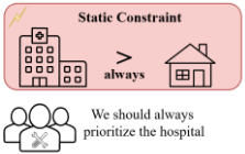
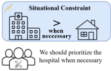
Traditional coordination methods often struggle with scalability in dynamic environments. While Reinforcement Learning (RL) has emerged as a robust alternative, existing algorithms for learning CEs [Zhang et al., 2023] are limited to static constraints. They lack the expressiveness to handle the logic implications required by context-dependent objectives. This raises a central question: How can we learn coordination policies that respect these dynamic, situational constraints?
In this paper, we propose Situational-Constrained DensityBased Correlated Equilibria (SC-DBCE), a solution concept that formalizes situational constraints as logical implications over state visitation distributions. To compute SC-DBCE, we develop the Situational-Constrained Correlated Policy Iteration (SC-CPI) algorithm. Unlike previous methods that unstably prioritize singular constraints, SC-CPI introduces a smooth Log-Sum-Exp aggregation mechanism. This allows the algorithm to optimize all atomic constraints simultaneously, ensuring stable convergence. To our knowledge, this is the first algorithm to solve multi-agent coordination under situational constraints.
We evaluate SC-CPI on the extended Multi-Agent Game benchmark [Zhang et al., 2023], and coordination benchmarks over smart grid scenarios as well as warehouse robot scenarios. In all environments, SC-CPI consistently outperforms baselines, achieving lower constraint violations and higher equilibrium quality.
We summarize our key contributions as follows:
- We propose SC-DBCE, a solution concept that extends existing correlated equilibria and accommodates contextsensitive coordination requirements in Markov Games.
- We develop SC-CPI, a reinforcement learning algorithm that effectively optimizes situational constraints via a smooth aggregation mechanism.
- We empirically demonstrate that SC-CPI outperforms existing baselines in satisfying situational constraints and computing high-quality correlated equilibria.
2 RelatedWork
Multi-Agent Coordination and Correlated Equilibrium. Multi-Agent coordination requires agents to align decisions toward collective objectives while respecting individual interests [Sun et al., 2025]. Applications range from V2V communication [Foerster et al., 2016] to warehouse robotics [Wurman et al., 2008]. Continual planning, one canonical approach, is effective in fully cooperative settings [Durfee et al., 1999; Torreno et al., ; Gonz´alez-Soto et al., 2025], it struggles to generalize to mixed-motive scenarios where agents have conflicting incentives. Game-theoretic approaches provide a robust alternative for such general interactions. Specifically, Correlated Equilibrium (CE) [Aumann, 1974] extends the Nash Equilibrium by allowing agents to coordinate via shared signals. This mechanism effectively models implicit coordination in systems like cognitive radio networks [Han et al., 2007] and smart grids [Yu et al., 2014]. Algorithms such as Correlated Q-learning [Greenwald et al., 2003] and entropy-regularized methods [Ortiz et al., 2007] have been developed to compute these equilibria efficiently. However, standard game-theoretical approaches often focus on the discussions over the tradeoff among agents' reward signals.
Constraints in Coordination. Besides the reward signal, constraints are also crucial for real-world deployment, such as safety and fairness [Garcıa and Fern´andez, 2015; Pu, 2021], leading to extensions of standard game models. To incorporate these properties, two primary streams of research have emerged. The first employs risk-sensitive utility functions [Markowitz, 1952], though these often suffer from ambiguity in parameter tuning. The second utilizes constrained optimization [Altman and Shwartz, 2000], but often requires expert knowledge in defining proper constraints. Recent works employ density function [Rantzer, 2001] to define constraints via state visitation distributions [Qin et al., 2021; Zhang et al., 2023]. This approach is advantageous not only for its clear physical interpretation as the long-term state distribution in Markov Games, but also for its mathematical tractability, specifically the one-to-one correspondence between state-action densities and joint policies. While the methods above discuss static constraints, some constraints are only applied based on context. Contextual models [Hallak et al., 2015; Sessa et al., 2020] provide a method for modeling such constraints by involving contextual variables. But they inherently handle multiple coordination problems under different contexts. [Zhang et al., 2025] recently addressed context-dependent situational constraints in a single MDP without involving additional information. However, it was restricted to single-agent settings. Our work fills this gap by leveraging situational constraints within a CE framework to address multi-agent coordination under context-sensitive properties via density functions.
3 ProblemFormulation
3.1 Multi-Agent coordination as Markov Games
The set of all natural numbers, reals, and non-negative reals are denoted by N, R, and R≥0, respectively. For a natural number N, the set {1, . . . ,N} is denoted by [N].
Markov Games [Littman, 1994] are extensions of Markov Decision Processes to the multi-agent setting, where a set of agents act in an environment, each aiming to maximize its cumulative rewards. The reward setting in the game can capture the mixed cooperative and competitive nature, thus making the Markov Game a suitable model for multi-agent coordination problems.
Definition 1. An N-agent Markov game is a tuple
- S is the set of states,
- Ai is the set of actions for the ith agent,
- P : S ×A→∆(S) is the transition function that specifies the transition probability between two states given a joint action a = (a1, . . . , an), where A = ×Ni=1Ai is the space of joint actions and ∆(S) denotes the set of probability distributions over S,
- ri : S×A→R is a reward function that determines agent i's immediate reward of a joint action in a state,
- η ∈ ∆(S) is the initial distribution of states,
- γ ∈ (0, 1) is a discount factor.
Definition 2. The agents' (stationary) joint policy is a function π : S → ∆(A) which specifies agents' probabilistic choice of actions according to the current state. The set of all joint policies is denoted by Π.
Given a joint policy π, the expected cumulative reward gained by each agent i from state s and joint action a is defined as:
3.2 Situational Constrained Density-Based Correlated Equilibrium
A solution to a Markov game is called an equilibrium, referring to a joint policy under which no agent has an incentive to unilaterally deviate to improve their expected reward. In this work, we focus on the Correlated Equilibrium (CE) [Aumann, 1987], which extends the classical Nash Equilibrium by allowing coordination among agents. This coordination is modeled via a correlation device that recommends an action ai ∈ Ai to each agent i, while revealing the conditional distribution π-i(a-i|s, ai) of the other agents' actions. A joint policy is a CE if no agent gains by deviating from the recommended action ai to any alternate action a′i ∈ Ai.
The incentive to deviate is measured by a quantity called regret, defined as the expected gain from unilaterally switching to a deviation action. Formally:
Definition 3. A correlated equilibrium (CE) for a Markov game is a joint policy π satisfying:
where the regret is defined as
The set of all CEs in a Markov game forms a convex polytope in the space of expected agent returns, as defined by the linear inequality constraints in Eq. (1). While any point in this set corresponds to a valid CE, not all are equally desirable in practice. In particular, real-world multi-agent tasks often involve additional state-dependent properties such as fairness, safety. In this paper, these properties are expressed using the density function [Rantzer, 2001], which measures how frequently each state is visited under a policy.
Formally, given an initial distribution η and a discount factor γ, the density function under a joint policy π is defined as:
For convenience, we define the density of a set of states as the sum of density of states in the set S∗ : ρπ (S∗ ) = ∑s∈S∗ ρπ (s). Enjoying a clear physical meaning, the density function can easily expresses the aforementioned properties. For instance, safety property can be forbidding visitation to unsafe states S′ , i.e., ρπ (S′ ) ≤ 0; and fairness can be balancing visitation frequency to two sets of states S1, S2, i.e., |ρπ (S1) - ρπ (S2)| ≤ 0.
Although the density function is powerful enough to address static constraints such as equity and safety [Zhang et al., 2023], we are interested in more complex situational constraints. In this paper, a situational constraint is constructed by a premise and a constraint, stating "If a premise holds, then a constraint must be applied." The Density-Based situational constraint was proposed to solve sequential resource allocation problems in single-agent systems, enabling the agent to adaptively allocate resources in varying environments [Zhang et al., 2025]. Here we define the situational constraints with density functions as follow:
Definition 4 (situational constraints with density function). Consider a Markov Game with m states. An atomic constraint is of the form⃗a · ⃗ ρπ ≤ b where vector ⃗a ∈ Rm and b ∈ R are parameters. A situational constraint is of the form φ1 → φ2, where φ1 and φ2 are atomic.
With the situational constraint, we propose a solution concept Situational-Constrained Density-Based Correlated Equilibria (SC-DBCE) as the CE satisfies a situational constraint most. This definition allows us to specify conditionaware solution concepts to multi-agent coordination tasks.
The examples below explain how situational constraints express condition-aware properties in a multi-agent coordination task:
Example 1 (Situational Constraint in Smart Grid). Consider a smart grid with multiple facilities, including a designated critical subset such as hospitals. Under normal operation, the objective is to supply all facilities, while under stress critical loads must be prioritised.
Let Sshort denote the set of states in which universal supply cannot be ensured (at least one facility lacks power), and let Scrit denote the set of states in which all critical facilities are supplied. Denote by ρπ (·) the long horizon state density under policy π. For thresholds c1, c2, the situational constraint is
This captures critical load protection: if shortages occur with density above c1, the policy must ensure that critical facilities receive power with density at least c2.
To find an SC-DBCE, we need an objective function represents the satisfaction of Ψ, i.e., the objective function leads to the least violation of Ψ. For a situational constraint Ψ and a policy π, we define the objective function as σ(Ψ, π). The formal definition of σ will be given in the next section. With such a function σ, we now are able to present our problem:
Definition 5. Let the following be given:
- AMarkov Game (S, {Ai}Ni=1 , P, {ri}Ni=1 , η, γ);
- A conjunction of situational constraints Ψ;
A joint policy π is called a Situational-Constrained DensityBased Correlated Equilibrium (SC-DBCE) if it is a solution to the following constrained optimization problem:
4 Method
4.1 Unification with OccupancyMeasure
Directly solving Problem 1 is intractable since the violation to a situational constraint depends on the densities of states, and the regret relies on the expected reward of a policy. Thus calculating an SC-DBCE needs a unification in the problem representation. Therefore, we may rewrite the Problem 1 based on the occupancy measure.
We introduce the occupancy measure µπ (s, a) [Syed et al., 2008], which defines the joint discounted visitation frequency over state-action pairs, to unify the situational constraint and regret. It is formally defined as:
and marginalizes to the state density via sum over actions.
The unification is done by an important property offered by occupancy measure: there is a one-to-one correspondence between a stationary policy π and an occupancy measure µπ , provided the latter satisfies the Bellman flow (BF) constraints:
Once a valid occupancy measure µ satisfying the BF constraints, a corresponding policy can be recovered via normalization: π(s, a) = µ(s, a) / ∑a′∈A µ(s, a′ ). In the later sections, we write µ to indicate the function which is an occupancy measure with corresponding policy is π.
Recall that a function µ is called an occupancy measure and owns a one-to-one correspondence to a policy π if it satisfies the Bellman flow constraint. Meanwhile, the density function of an occupancy measure can be easily derived by taking sum over actions. Thus, solving a policy which is a CE can be reformulated as solving an occupancy measure whose corresponding policy is a CE. The resulting problem is shown below, where σ(Ψ, µ) is the objective function representing the violation of the situational constraint of µ, and reg′µ is the regret of corresponding policy to µ.
Comparing the Problem 2 with Problem 1, we can now focus on solving a single term µ, and obtain a CE by calculating its corresponding policy. However, this problem still cannot be directly solved. Although the Bellman Flow constraints in eq. 4 and eq. 5 directly rely on µ, there are still two challenges. First, the regret still requires solving the expected reward of the corresponding policy of µ; Second, we need to define a proper objective function to find SC-DBCE.
Here, we introduce a framework that solves the first challenge. It interchangeably updates the evaluated values Q according to the current policy; and the corresponding policy π of µ. The framework is shown in Alg. 1, which is devoted to finding CEs to a Markov Game.
The algorithm framework iterates through two steps:
- Policy optimization via occupancy measure: In the outer loop, the algorithm solves an optimization problem (Problem 2) to obtain the current occupancy measure µ, with corresponding policy π. The objective function σ is user-defined and specifies the desired properties of π, e.g., max entropy or max social welfare.
- Q-function evaluation: In the inner loop, the Q-functions {Qi}Ni=1 are updated under the current policy π. This provides updated value estimates for regret computation in the next round of occupancy measure optimization.
Algorithm 1 Algorithm Framework: Finding CE
- 1: Input: A Markov game (S,A, P, {ri}Ni=1 , η, γ), and an objective function σ(Ψ, µ)
- 2: Initialize: Occupancy measure µ, Q-functions Qi for each i ∈ [N], learning rate α
- 3: for each iteration do
- 4: Solve for µ by optimizing the objective σ(Ψ, µ) subject to the Problem 2
- 5: Derive policy π from µ via normalization: π(s, a) = µ(s, a)/ ∑a′∈A µ(s, a′ )
- 6: while not converged do
- 7: Sample transitions (s, a, r, s′ )
- 8: Evaluate Qi for each i ∈ [N]
- 9: end while
- 10: end for
- 11: Output: Joint policy π, final objective value σ(µ)
This iterative process continues until convergence, and its behavior is determined by the choice of the objective function σ. For instance, uCE-Q [Greenwald et al., 2003] can be viewed as an instantiation of this framework where the objective σ is defined by sum of rewards, aiming to find a CE that maximizes total return without considering statevisitation structure. In contrast, theDensity-BasedCorrelated Policy Iteration (DBCPI) [Zhang et al., 2023] algorithm also fits into this framework but specifies σ(µ) as a static DensityBased function. Now it lefts to define a proper σ to handle the situational constraints, i.e., developing an algorithm finds SC-DBCE.
4.2 Handling Situational Constraint
To evaluate constraint satisfaction under a given policy π, we define the violation of an atomic constraint φ : ⃗a · ⃗ ρπ ≤ b as V ioπ (φ) :=⃗a· ⃗ ρπ -b [Zhang et al., 2025], where ⃗ ρπ denotes the density function induced by π. This quantity measures the extent to which the policy exceeds the constraint threshold, with non-positive values indicating satisfaction. In practice, the density ⃗ ρπ is derived from the occupancy measure µ by marginalizing over joint actions: ρπ (s) = ∑a∈A µ(s, a).
To capture logical dependencies, we rewrite the situational constraints in implications ψ := φ1 → φ2 as disjunctions ¬φ1 ∨ φ2 due to the equivalence between these two forms. A policy violates ψ only if it fails to satisfy both disjuncts. Thus, the violation can be defined as V ioπ (ψ) := min{V ioπ (¬φ1), V ioπ (φ2)}, where violation is zero if either sub-constraint is satisfied. This recursive structure allows us to compute violation magnitudes for complex logical constraints in a consistent manner.
Designing the objective function σ(µ) is essential to solving Problem 2, as it quantifies the degree to which a policy violates logical constraints. To be valid, σ should be nonnegative and equal to zero when all constraints are satisfied. The most direct way to handle situational constraints in the form ψ = φ1 → φ2, is to decompose them into disjunctive normal form (DNF) and optimize each disjunct separately. This results in multiple subproblems corresponding to the two satisfaction branches of the implication, can be written in minimizing Vioπ (¬φ1) and Vioπ (φ2) independently, each of which can be handled by existing CE-solving methods such as DBCPI [Zhang et al., 2023]. While semantically clear and easy to implement, this approach is computationally expensive, as the number of disjuncts increases rapidly with the complexity of the constraint.
To avoid combinatorial overhead, recent works have explored unified formulations that directly define σ(µ) = Vioπ (ψ) using semantics of the disjunctive form. A common choice is to use the minimum operator [Ren et al., ; Huang et al., 2022], i.e., Vioπ (ψ) = min{Vioπ (¬φ1),Vioπ (φ2)}, or probabilistic selection to prioritize less-violated subformula [Zhang et al., 2025]. However, both approaches suffer from instability in optimization direction. Since each CEsolving step involves constrained optimization, large fluctuations in σ(µ) across iterations can destabilize convergence, impeding the algorithm from finding a CE. Therefore, a more stable objective design is needed to ensure consistent and reliable optimization under disjunctive constraints.
To address the instability caused by disjunctive constraints in the optimization objective, we adopt the LogSum-Exp (LSE) technique to smooth the original optimization objective. Specifically, for a situational constraint ψ = φ1 ∨ φ2, the ideal objective function min{Vioπ (φ1),Vioπ (φ2)} is first reformulated with max operator as -max{-Vioπ (φ1),-Vioπ (φ2)}, and then approximated using the standard LSE transformation:
where β > 0 controls the approximation sharpness. The LogSum-Exp function provides a smooth, differentiable approximation to the max operator, and is widely used in convex optimization due to its favorable analytical properties. Compared to earlier approaches that either directly minimize the minimum violation or randomly select sub-formulas during optimization, this formulation avoids explicitly committing to a single disjunct at each iteration. As a result, it offers a stable optimization direction throughout training, which greatly improves convergence behavior. Moreover, since LSE closely approximates the true violation semantics under disjunction, it faithfully preserves the intent of the original situational constraint while enabling efficient gradient-based optimization.
Formally, given an occupancy measure µ and its corresponding policy π, the objective function σ(·, µ) is defined recursively as follows. For an atomic constraint φ : ⃗a · ⃗ ρπ ≤ b, we define σ(φ, µ) :=⃗a· ⃗ ρπ -b. For a situational constraint of the form ψ := φ1 → φ2, the violation is computed as σ(ψ, µ) := - 1β log (exp(-β · σ(¬φ1, µ)) + exp(-β · σ(φ2, µ))) ,
where β > 0 is a temperature parameter controlling the approximation sharpness. Finally, for a conjunction of constraints Ψ := ∧ki=1 ψi, we compute the total violation as the sum over individual components: σ(Ψ, µ) := ∑ki=1 σ(ψi, µ).
4.3 Algorithm
Building on the above definition of σ(µ), we now proceed to develop an algorithm Situational-Constrained Correlated Policy Iteration (SC-CPI) tailored to finding situationalconstrained correlated equilibria (SC-DBCE). The central idea is to embed the violation-aware objective σ(µ) into a policy iteration framework, where policy optimization is conducted over the occupancy measure space rather than the space of joint policies directly. This transformation enables us to naturally encode both logical constraints and equilibrium conditions within a single convex optimization problem (Problem 2). However, the regret term and value estimates within the constraint set still depend on the Q-values associated with the current policy. We address this by using an iterative scheme that alternates between optimizing the occupancy measure under fixed Q-functions and performing policy evaluation to update Q-values under the current policy, i.e., Qi(s, a) ← (1 - α)Qi(s, a) + α(ri + γVi(s′ )). The resulting procedure is formally outlined as follows.
The following theorem shows that the Alg. 2 converges to a CE as a solution to the Prob. 2.
Assumption 1. Each state s ∈ S and action ai ∈ Ai for all i ∈ [N] are visited infinitely often.
Assumption 2. The reward is bounded by some constant.
Assumption 3. The learning rate αt satisfies the following conditions: 0 ≤ αt < 1 ∀t, ∑t αt = ∞ and ∑t α2 t <∞.
Theorem 1 ([Zhang et al., 2023]). Under Assumption 1-3, the Q function iteratively updated in Alg. 2 will converge to the one under a CE if for all t, s ∈ S, and i ∈ [N], the policy πt is recognized as the global optimum expressed as:
Proof. The intuition is to show that the policy guided by SCCPI monotonically increases in terms of reward. Meanwhile, at each iteration, the optimization problem reformulated by LSE transformation can be solved by any existing optimizer, thus satisfying the constraints in Prob. 2.
Algorithm 2 Situational-Constrained Correlated Policy Iteration (SC-CPI)
- 1: Input: Markov game (S,A, P, {ri}Ni=1 , η, γ), and objective function σ(Ψ, µ) defined over a situational constraintΨ.
- 2: Initialize: Occupancy measure µ, Q-functions Qi for each agent i ∈ [N], and learning rate α.
- 3: for each outer iteration do
- 4: Solve Problem2 to obtain the occupancymeasure µ by minimizing σ(Ψ, µ), subject to CE and Bellman flow constraints.
- 5: Derive the joint policy π from µ.
- 6: while policy evaluation not converged do
- 7: Sample transitions (s, a, r, s′ ) from environment under policy π.
- 8: Update Q-function Qi for each agent i ∈ [N].
- 9: Decay learning rate α
- 10: end while
- 11: end for
- 12: Output: Joint policy π.
5 Experiment
We aim to validate SC-CPI algorithm's performance through empirical evaluations over two multi-agent coordination scenarios. Code is available in the supplement.
5.1 Experiment Scenarios and Tasks
Our evaluation comprises two parts: a reproduction of the Multi-Agent Game Benchmark [Zhang et al., 2023] and two complex Coordination Scenarios. All environments are modeled as discrete Markov games with a discount factor γ = 0.99.
Multi-Agent Game Benchmark. We adopt three environments from [Zhang et al., 2023], extending them with situational constraints to validate SC-DBCE. 1. Fair Gamble: A risk-management scenario where agents select among tables with varying reward variances. We impose a constraint requiring that if the system enters high-risk states frequently, it must also maintain a significant density of low-risk states to balance the overall risk profile. 2. Collect and Explore (CaE): A fully cooperative task involving resource gathering and exploration. The situational constraint promotes synchronization: if a specific protected agent initiates exploration, other agents are required to explore concurrently rather than acting in isolation. 3. Hunters: A mixed cooperativecompetitive scenario involving village guarding versus prey hunting. To ensure safety, the constraint dictates that if the village is left completely unguarded beyond a safety threshold, the agents must offset this by maintaining a high frequency of fully guarded states.
Coordination Benchmarks. We further evaluate SC-CPI on two practical domains requiring complex resource allocation and path planning. 1. Smart Grid [Zhang et al., 2024]: This scenario models a grid operator managing two repair teams to protect one critical facility and two residential communities from power outages. The situational constraint enforces a resilience protocol: if a broad "sufficient protection" standard (covering all facilities) cannot be met due to high failure rates, the agents must strictly prioritize "critical load protection" for the infrastructure site, effectively sacrificing peripheral coverage to prevent catastrophic failure. 2. Warehouse: This environment involves two robots navigating parallel corridors to retrieve and deliver cargo from shared and private shelves. The constraint manages the trade-off between efficiency and congestion: if the frequency of conflicts (simultaneous delivery in the same corridor) exceeds a tolerance threshold, the agents are required to maintain a high density of parallel, non-conflicting operations in separate corridors to recover system throughput.
5.2 Baselines
We compare our approach against three baseline methods:
- Utilitarian Correlated Q Learning (uCE-Q) [Greenwald et al., 2003]. uCE-Q learns a CE with maximizing the sum of rewards as an objective function. It serves as a utilitarian baseline without considering density functionspecified objectives.
- Density-Based Correlated Policy Iteration (DBCPI) [Zhang et al., 2023]. DBCPI finds DensityBased CEs without the ability to handle situational constraints. So we decompose each situational constraint φ1 → φ2 into: (DBCPI-1): the negation of the premise ¬φ1 and (DBCPI-2): The conclusion φ2.
- Probabilistic DBCPI (Prob-DBCPI) [Zhang et al., 2025]. We implement the probabilistic mechanism from SCRL [Zhang et al., 2025] into the DBCPI framework as a baseline. The Prob-DBCPI selects the sub-formula in a situational constraint with probabilities based on the violation degree in each iteration.
5.3 Performance Metrics
The primary evaluation metric, constraint violation (Cons.Vio.), measures violation of constraints. A lower Cons.Vio. indicates better compliance with these critical constraints and is preferred. The second evaluation metric, maximum regret (MaxReg), measures the max regret among all agents' state-action pairs. A low MaxReg indicates the resulting policy is closer to the CE set. The last evaluation metric, Bellman Flow Error (BFErr), measures the value of Bellman Flow Error. A low BFErr indicates the result is more reliable since correspondence between the policy and occupancy measure is retained.
5.4 Experiment Result
Table 1 presents the results. Regarding constraint violation, uCE-Q fails in WAREHOUSE due to lacking explicit constraint modeling, while Prob-DBCPI shows widespread violations due to unstable optimization. DBCPI satisfies constraints only partially via independent instances. In contrast, SC-CPI consistently achieves near-zero violation, highlighting its effectiveness. Regarding equilibrium quality (MaxReg), uCE-Q shows high regret in HUNTERS, and ProbDBCPI performs poorly across multiple scenarios, indicating non-CE policies. For Bellman flow error (BFErr), all baselines incur large errors in SMART GRID, whereas SC-CPI maintains low error, confirming its robustness.
Overall, these results show that SC-CPI has advantages in both satisfying situational constraints and stably producing equilibria against the existing baselines.
Case Study: More Disjuncts. Table 2 evaluates performance under a complex constraint with four independent disjuncts. While the loose logical requirement, where satisfying any single disjunct suffices, reduces violation rates, the increased structural complexity destabilizes learning. Consequently, SC-CPI's Bellman Flow error rises to 1.19. However, this remains the lowest among all baselines, confirming that SC-CPI maintains its robustness advantage even under complex optimization landscapes. In conclusion, a complex situational constraint is more challenging, but the advantage of SC-CPI against other baselines remains.
Case Study: Learning Stability. The stability performance of different algorithms in Smart Grid environment is shown in Figure 2. Overall, Figure 2a plots the regret curves, where most algorithms exhibit a typical pattern: high initial regret followed by a rapid decline and eventual stabilization. This aligns with standard reinforcement learning dynamics, where both the Q-function and policy gradually converge. However, such convergence behavior is notably absent in Prob-DBCPI.
| Method | Cons.Vio. | MaxReg | BFErr |
|---|---|---|---|
| Scenario: Fair Gamble | |||
| uCE-Q | 0.00 ± 0.00 | 0.02 ± 0.02 | 0.20 ± 0.23 |
| DBCPI-1 | 0.00 ± 0.00 | 0.00 ± 0.01 | 0.05 ± 0.08 |
| DBCPI-2 | 23.66 ± 24.65 | 0.05 ± 0.06 | 0.56 ± 0.63 |
| Prob-DBCPI | 0.00 ± 0.00 | 0.00 ± 0.00 | 0.00 ± 0.01 |
| SC-CPI | 0.00 ± 0.00 | 0.01 ± 0.02 | 0.16 ± 0.25 |
| Scenario: CaE | |||
| uCE-Q | 0.00 ± 0.00 | 0.00 ± 0.00 | 0.00 ± 0.00 |
| DBCPI-1 | 19.83 ± 20.88 | 0.00 ± 0.00 | 0.00 ± 0.00 |
| DBCPI-2 | 0.00 ± 0.00 | 0.00 ± 0.00 | 0.00 ± 0.00 |
| Prob-DBCPI | 4.44 ± 3.56 | 8.20 ± 8.92 | 1.39 ± 0.84 |
| SC-CPI | 0.00 ± 0.00 | 0.00 ± 0.00 | 0.00 ± 0.00 |
| Scenario: Hunters | |||
| uCE-Q | 0.72 ± 1.18 | 3.95 ± 4.87 | 0.00 ± 0.00 |
| DBCPI-1 | 0.00 ± 0.00 | 0.00 ± 0.01 | 0.00 ± 0.00 |
| DBCPI-2 | 8.11 ± 17.61 | 0.06 ± 0.13 | 0.01 ± 0.03 |
| Prob-DBCPI | 3.09 ± 0.30 | 10.99 ± 0.96 | 0.17 ± 0.18 |
| SC-CPI | 0.41 ± 0.92 | 0.00 ± 0.00 | 0.00 ± 0.00 |
| Scenario: Warehouse | |||
| uCE-Q | 23.94 ± 2.23 | 0.11 ± 0.05 | 0.02 ± 0.01 |
| DBCPI-1 | 42.27 ± 0.11 | 0.09 ± 0.03 | 0.02 ± 0.00 |
| DBCPI-2 | 8.73 ± 4.71 | 0.16 ± 0.07 | 0.02 ± 0.00 |
| Prob-DBCPI | 9.17 ± 6.87 | 0.78 ± 0.94 | 0.34 ± 0.39 |
| SC-CPI | 8.02 ± 2.75 | 0.10 ± 0.02 | 0.03 ± 0.00 |
| Scenario: Smart Grid | |||
| uCE-Q | 0.00 ± 0.00 | 0.30 ± 0.05 | 2.94 ± 0.27 |
| DBCPI-1 | 0.33 ± 0.75 | 0.20 ± 0.13 | 2.09 ± 1.20 |
| DBCPI-2 | 0.73 ± 1.63 | 0.31 ± 0.03 | 2.72 ± 0.27 |
| Prob-DBCPI | 4.97 ± 3.39 | 2.96 ± 0.27 | 26.01 ± 2.49 |
| SC-CPI | 0.00 ± 0.00 | 0.03 ± 0.03 | 0.27 ± 0.32 |
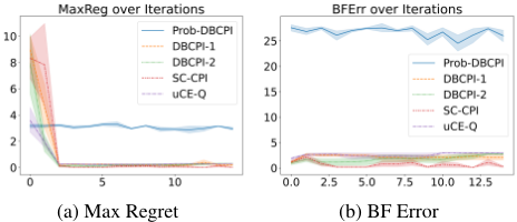
Figure 2b shows the BF-Err curves. Most algorithms maintain low BF-Err over time, but Prob-DBCPI consistently exhibits high BF-Err, indicating its failure to produce reliable occupancy measures. These results highlight that the probabilistic mechanism used to handle situational constraints is ill-suited for computing correlated equilibria. In contrast, SCCPI effectively addresses this issue by applying a log-sumexp (LSE) approximation to the objective function, ensuring stability while respecting situational constraints.
| Method | Cons.Vio. | MaxReg | BFErr |
|---|---|---|---|
| uCE-Q | 0.00 ± 0.00 | 0.37 ± 0.18 | 2.96 ± 0.15 |
| DBCPI-1 | 0.02 ± 0.05 | 0.19 ± 0.17 | 1.69 ± 1.52 |
| DBCPI-2 | 0.00 ± 0.00 | 0.20 ± 0.13 | 1.98 ± 1.32 |
| DBCPI-3 | 14.77 ± 3.79 | 0.16 ± 0.14 | 1.60 ± 1.35 |
| DBCPI-4 | 0.00 ± 0.00 | 0.18 ± 0.15 | 1.75 ± 1.40 |
| Prob-DBCPI | 0.00 ± 0.00 | 0.31 ± 0.34 | 1.94 ± 1.63 |
| SC-CPI | 0.00 ± 0.00 | 0.12 ± 0.11 | 1.19 ± 1.09 |
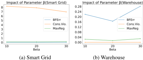
Parameter Study. To evaluate the impact of β in LSE transformation, we perform experiments with β from {10, 20(default), 30}. The result of Warehouse scenario is shown in Figure 3. We observe a slight decrease in constraint violation in Figure 3a, and consistent performance on the MaxReg and BFErr in two scenarios. Overall, the algorithm performs consistently under varying β.
6 Conclusion and Limitations
This paper solves multi-agent coordination problems under situational constraints. We model the problem as Markov Games and propose Situational-Constrained Density-Based Correlated Equilibria as solution concepts. We develop SCCPI as the first RL algorithm capable of finding such equilibria under context-sensitive objectives. Our work points a promising path by formalizing situational constraints in multi-agent systems, which is particularly critical for safetycritical infrastructures, such as autonomous traffic or smart grids, where constraints are dynamic and adherence to emergency protocols is as important as efficiency.
Limitations. Our approach still computes a joint policy, which may limit scalability in larger systems. Future work could explore fully decentralized methods or CTDE (Centralized Training with Decentralized Execution) frameworks to improve applicability in large-scale multi-agent settings.
@inproceedings{ijcai2026p53,
  title     = {Context-Aware Multi-Agent Coordination: Learning Correlated Equilibria Under Situational Constraints},
  author    = {Zhang, Libo and Zeng, Zhirui and Chen, Yang and Liu, Jiamou},
  booktitle = {Proceedings of the Thirty-Fifth International Joint Conference on
               Artificial Intelligence, {IJCAI-26}},
  publisher = {International Joint Conferences on Artificial Intelligence Organization},
  editor    = {Diego Calvanese},
  pages     = {463--471},
  year      = {2026},
  month     = {8},
  note      = {Main Track},
  doi       = {10.24963/ijcai.2026/53},
  url       = {https://doi.org/10.24963/ijcai.2026/53},
}
TY - CPAPER TI - Context-Aware Multi-Agent Coordination: Learning Correlated Equilibria Under Situational Constraints AU - Zhang, Libo AU - Zeng, Zhirui AU - Chen, Yang AU - Liu, Jiamou T2 - Proceedings of the Thirty-Fifth International Joint Conference on Artificial Intelligence, IJCAI-26 PB - International Joint Conferences on Artificial Intelligence Organization PY - 2026 SP - 463 EP - 471 DO - 10.24963/ijcai.2026/53 UR - https://doi.org/10.24963/ijcai.2026/53 ER -Copied
Machine-readable versions of this paper, for tools and AI agents:





