
Accelerated Distributed Riemannian Optimization Algorithms with Random Shuffling
Proceedings of the Thirty-Fifth International Joint Conference on Artificial Intelligence. Main Track. Pages 5083-5091.
https://doi.org/10.24963/ijcai.2026/566
Keywords
- Machine Learning: Federated learning
Abstract
Riemannian optimization has attracted increasing attention recently as it is related to a variety of machine learning problems, including principal component analysis, dictionary learning, and mixture modeling. To tackle modern large-scale machine learning tasks, distributed learning is usually considered as an effective solution that trains a global model over multiple worker nodes collaboratively to enhance the computational power. Centralized learning and decentralized learning are two types of distributed learning. Centralized learning employs a central parameter server to coordinate the training process while in decentralized learning, each worker only communicates with its peer neighbors. In this paper, we propose accelerated distributed Riemannian stochastic gradient descent algorithms with random shuffling in the cases of both centralized and decentralized learning. We improve the stochastic first-order oracle complexity of the Riemannian SGD from to where is the size of training data. We conduct an experiment of the leading eigenvector problem under the condition of centralized learning and decentralized learning to validate the performance of our methods.
- [Arjovsky et al., 2016] Martin Arjovsky, Amar Shah, and Yoshua Bengio. Unitary evolution recurrent neural net- works. International conference on machine learning, 48:1120-1128, 2016.
- [Bonnabel, 2013] Silvere Bonnabel. Stochastic gradient de- scent on riemannian manifolds. IEEE Transactions on Au- tomatic Control, 58(9):2217-2229, 2013.
- [Bottou, 2009] Léon Bottou. Curiously fast convergence of some stochastic gradient descent algorithms. Proceedings of the symposium on learning and data science, 8:2624- 2633, 2009.
- [Chen et al., 2021] Shixiang Chen, Alfredo Garcia, Mingyi Hong, and Shahin Shahrampour. Decentralized rieman- nian gradient descent on the stiefel manifold. International Conference on Machine Learning, 139:1594-1605, 2021.
- [Cherian and Sra, 2016] Anoop Cherian and Suvrit Sra. Rie- mannian dictionary learning and sparse coding for positive definite matrices. IEEE transactions on neural networks and learning systems, 28(12):2859-2871, 2016.
- [Ghadimi and Lan, 2013] Saeed Ghadimi and Guanghui Lan. Stochastic first-and zeroth-order methods for non- convex stochastic programming. SIAM journal on opti- mization, 23(4):2341-2368, 2013.
- [Grammenos et al., 2020] Andreas Grammenos, Rodrigo Mendoza Smith, Jon Crowcroft, and Cecilia Mascolo. Federated principal component analysis. Advances in neu- ral information processing systems, 33:6453-6464, 2020.
- [Haochen and Sra, 2019] Jeff Haochen and Suvrit Sra. Ran- dom shuffling beats sgd after finite epochs. International Conference on Machine Learning, 97:2624-2633, 2019.
- [Hosseini and Sra, 2015] Reshad Hosseini and Suvrit Sra. Matrix manifold optimization for gaussian mixtures. Ad- vances in neural information processing systems, 28:910- 918, 2015.
- [Huang et al., 2018] Lei Huang, Xianglong Liu, Bo Lang, Adams Yu, Yongliang Wang, and Bo Li. Orthogonal weight normalization: Solution to optimization over mul- tiple dependent stiefel manifolds in deep neural networks. Proceedings of the AAAI Conference on Artificial Intelli- gence, 32(1):3271-3278, 2018.
- [Kasai et al., 2018] Hiroyuki Kasai, Hiroyuki Sato, and Bamdev Mishra. Riemannian stochastic recursive gradient algorithm. International conference on machine learning, 80:2516-2524, 2018.
- [Li and Ma, 2022] Jiaxiang Li and Shiqian Ma. Feder- ated learning on riemannian manifolds. arXiv preprint arXiv:2206.05668, 2022.
- [Lian et al., 2015] Xiangru Lian, Yijun Huang, Yuncheng Li, and Ji Liu. Asynchronous parallel stochastic gradient for nonconvex optimization. Advances in neural information processing systems, 28:2737-2745, 2015.
- [Lian et al., 2017] Xiangru Lian, Ce Zhang, Huan Zhang, Cho-Jui Hsieh, Wei Zhang, and Ji Liu. Can decentral- ized algorithms outperform centralized algorithms? a case study for decentralized parallel stochastic gradient de- scent. Advances in Neural Information Processing Sys- tems, 30:5330-5340, 2017.
- [Liu et al., 2003] Xiuwen Liu, Anuj Srivastava, and Kyle Gallivan. Optimal linear representations of images for object recognition. IEEE Computer Society Conference on Computer Vision and Pattern Recognition, 1:229-234, 2003.
- [Liu et al., 2019] Huikang Liu, Anthony Man-Cho So, and Weijie Wu. Quadratic optimization with orthogonality constraint: explicit łojasiewicz exponent and linear con- vergence of retraction-based line-search and stochastic variance-reduced gradient methods. Mathematical Pro- gramming, 178(1):215-262, 2019.
- [Meng et al., 2019] Qi Meng, Wei Chen, Yue Wang, Zhi- Ming Ma, and Tie-Yan Liu. Convergence analysis of dis- tributed stochastic gradient descent with shuffling. Neuro- computing, 337:46-57, 2019.
- [Mishchenko et al., 2020] Konstantin Mishchenko, Ahmed Khaled, and Peter Richtárik. Random reshuffling: Sim- ple analysis with vast improvements. Advances in Neural Information Processing Systems, 33:17309-17320, 2020.
- [Mishchenko et al., 2022] Konstantin Mishchenko, Ahmed Khaled, and Peter Richtarik. Proximal and federated random reshuffling. Proceedings of the 39th Interna- tional Conference on Machine Learning, 162:15718- 15749, 2022.
- [Nagaraj et al., 2019] Dheeraj Nagaraj, Prateek Jain, and Praneeth Netrapalli. Sgd without replacement: Sharper rates for general smooth convex functions. International Conference on Machine Learning, 97:4703-4711, 2019.
- [Nguyen et al., 2021] Lam M Nguyen, Quoc Tran-Dinh, Dzung T Phan, Phuong Ha Nguyen, and Marten Van Dijk. A unified convergence analysis for shuffling-type gradi- ent methods. Journal of Machine Learning Research, 22(207):1-44, 2021.
- [Rajput et al., 2020] Shashank Rajput, Anant Gupta, and Dimitris Papailiopoulos. Closing the convergence gap of sgd without replacement. International Conference on Machine Learning, 119:7964-7973, 2020.
- [Safran and Shamir, 2020] Itay Safran and Ohad Shamir. How good is sgd with random shuffling? Conference on Learning Theory, 125:3250-3284, 2020.
- [Shah, 2017] Suhail M Shah. Distributed optimization on riemannian manifolds for multi-agent networks. arXiv preprint arXiv:1711.11196, 2017.
- [Shamir, 2016] Ohad Shamir. Without-replacement sam- pling for stochastic gradient methods. Advances in neural information processing systems, 29:46-54, 2016.
- [Sun et al., 2016] Ju Sun, Qing Qu, and John Wright. Com- plete dictionary recovery over the sphere ii: Recovery by riemannian trust-region method. IEEE Transactions on In- formation Theory, 63(2):885-914, 2016.
- [Tang et al., 2018] Hanlin Tang, Xiangru Lian, Ming Yan, Ce Zhang, and Ji Liu. d 2 : Decentralized training over decentralized data. Proceedings of the 35th International Conference on Machine Learning, 80:4848-4856, 2018.
- [Wold et al., 1987] Svante Wold, Kim Esbensen, and Paul Geladi. Principal component analysis. Chemometrics and intelligent laboratory systems, 2:37-52, 1987.
- [Zhang and Sra, 2016] Hongyi Zhang and Suvrit Sra. First- order methods for geodesically convex optimization. Con- ference on learning theory, 49:1617-1638, 2016.
- [Zhang et al., 2016] Hongyi Zhang, Sashank J Reddi, and Suvrit Sra. Riemannian svrg: Fast stochastic optimization on riemannian manifolds. Advances in Neural Information Processing Systems, 29:4592-4600, 2016.
- [Zhou et al., 2019] Pan Zhou, Xiao-Tong Yuan, and Jiashi Feng. Faster first-order methods for stochastic non-convex optimization on riemannian manifolds. The 22nd Interna- tional Conference on Artificial Intelligence and Statistics, 89:138-147, 2019.
References were extracted automatically from the PDF and may contain errors.
Full text extracted automatically from the PDF; figures, tables and equations may differ. The PDF is the version of record.
1 Introduction
Optimization on Riemannian manifolds has received significant attention in recent years because it is the key issue of many machine learning problems, such as principal component analysis (PCA) [Wold et al., 1987], dictionary learning [Cherian and Sra, 2016; Sun et al., 2016], mixture modeling [Hosseini and Sra, 2015], and deep neural networks with orthogonal constraints [Arjovsky et al., 2016; Huang et al., 2018]. As an example, the principal component analysis results in a Riemannian optimization problem over the Stiefel manifold. One straightforward solution to the Riemannian optimization problem is to operate the projection onto the manifold. However, the projection computation could be too expensive. An alternative solution is to directly perform the optimization process on the manifold. The standard stochastic gradient descent on the Riemannian manifold was proposed in [Bonnabel, 2013] which computes the Riemannian gradients and adopts a retraction operation to map the tangent space to the manifold. More details of related works will be introduced in the next section.
In addition, distributed learning has emerged as a promising research area in the machine learning community. In distributed learning, multiple worker nodes collaboratively train a global learning model without sharing training data. Since large-scale data are distributed to different nodes and heavy computation workloads can be done in parallel, distributed learning is capable of tackling challenging large-scale learning tasks effectively and efficiently. There are two categories of distributed learning, centralized learning, and decentralized learning. Centralized learning is the classic distributed learning scheme that uses a central parameter server to efficiently coordinate the training process. The central node aggregates the computed results from worker nodes and broadcasts the new global model. In contrast, decentralized learning does not need a central node, and communication is only required between local neighborhoods. Decentralized learning has attracted more interest recently because it avoids the high communication overhead on the central node.
In this paper, we consider the following distributed optimization problem:
where M is the Stiefel manifold St(d, r) = {x ∈ Rd×r : xT x = Ir}. n is the number of worker nodes and K is the size of data on each node. fi is the local objective function on the i-th worker node, which is the finite sum of loss functions over Ki local training samples. Let N be the total number of training samples over all worker nodes. In this paper fi is supposed to be Lipschitz smooth and potentially (geodesically) nonconvex.
Due to the crucial importance of Riemannian optimization and distributed learning, we are motivated to study and accelerate the convergence rate of current distributed Riemannian stochastic gradient descent algorithms. We only consider stochastic algorithms because the full gradient is too expensive to compute for large data. Besides, the objective function is not necessarily convex because modern machine learning models are complicated and convexity cannot be guaranteed. Thus, in this paper we propose the centralized and decentralized distributed Riemannian stochastic gradient descent algorithms with random shuffling to improve the convergence rate for nonconvex Riemannian optimization. Random shuffling is the without-replacement version of SGD, which randomly shuffles the dataset in each epoch and loads the training data batch by batch sequentially, rather than using the vanilla with-replacement SGD. SGD with random shuffling converges faster in empirical [Bottou, 2009] and it can be computationally more practical [Bonnabel, 2013]. These reasons motivate us to study Riemannian optimization algorithms with random shuffling. In this paper, we establish a complete convergence analysis that covers both the conditions of centralization and decentralization to prove the advantages of our methods theoretically. We summarize our contributions as follows.
- We propose the centralized and decentralized distributed Riemannian stochastic gradient descent algorithms with random shuffling to accelerate the convergence rate of the standard SGD on Riemannian manifold.
- We establish the convergence analysis that covers both the conditions of centralized and decentralized learning, which guarantees the SFO complexity of O(√Nϵ-3 ) for nonconvex Riemannian optimization, where N is the size of training data. Our results match the best complexity of random shuffling SGD in Euclidean space.
- We conduct an experiment of the leading eigenvector problem to validate the performance of our methods.
2 Preliminary
2.1 Riemannian Optimization
As defined in problem (1), M denotes the Stiefel manifold. The notation TxM represents the tangent space at the point x on the manifold. In first-order Riemannian optimization algorithms [Bonnabel, 2013; Zhang and Sra, 2016], the Riemannian gradient is computed, which is defined by grad h(x) = PTxM∇h(x) where ∇h(x) is the gradient in the Euclidean space and PTxM is the orthogonal projection onto tangent space TxM. To map a vector v in the tangent space onto the manifold, in some early works the exponential map Expx : TxM → M is used, which finds a geodesic curve γ such that γ(0) = x and d dt γ(0) = v. However, in many circumstances the computation of the exponential map could be expensive. To avoid this issue, in recent works about Riemannian optimization, an approximated version called retraction map is used instead of the exponential map, which can be calculated much easier and faster. In each iteration of these algorithms, the update rule is defined by xt+1 = Rxt (-η grad h(xt)) where η is the learning rate and Rx is the retraction map. The retraction Rx : TxM → M is a map from the tangent space to the manifold with a local rigidity condition that preserves the gradient at x ∈ M. Moreover, we assume Rx is a second-order retraction such that Rx(u) = x+u+O(∥u∥2 ). In this paper, ∥ · ∥ represents the Frobenius norm if there is no special comment. We can achieve the following lemma, which ensures a bound of the gap between (x + u) and Rx(u).
Lemma 1. (Appendix E in [Liu et al., 2019]) Let R be a second-order retraction on Stiefel manifold M. Then for ∀x ∈ M and ∀u ∈ TxM, we have ∥Rx(u) - (x + u)∥ ≤ M∥u∥2 for some constant M. Especially, when we use polar retraction and ∥u∥ ≤ 1, we can set M = 1.
Asymptotic [Liu et al., 2003; Bonnabel, 2013] and nonasymptotic [Kasai et al., 2018] convergence analyzes were performed for previous Riemannian stochastic gradient descent algorithms for (geodesically) nonconvex problems. In [Kasai et al., 2018], the stochastic first-order oracle (SFO) of O(ϵ-4 ) was proved for the Riemannian stochastic gradient descent algorithm to achieve an ϵ-stationary point such that E∥grad f(x)∥ ≤ ϵ. Some subsequent works adopt variance reduction to accelerate the convergence rate of Riemannian stochastic gradient descent [Zhang et al., 2016; Zhou et al., 2019]. In this paper, we do not consider the variance reduction technique because the full gradient is required periodically in variance reduced algorithms, which will be expensive to compute when the size of data is large. Therefore, we only focus on the standard Riemannian stochastic gradient descent, which is more efficient and convenient to implement in practice.
2.2 Decentralized Optimization
Decentralized optimization is a class of distributed optimization that trains models in parallel across multiple worker nodes over a decentralized communication network. Different from the conventional centralized paradigm where all worker nodes need to communicate with the central node, in decentralized optimization each worker node only communicates with its neighbors, which avoids high communication cost issue on the central node, especially when the number of nodes is large. Furthermore, it has been shown that decentralized algorithms can achieve competitive convergence rates compared to their centralized counterparts [Lian et al., 2017; Tang et al., 2018].
In decentralized optimization, each worker node has its own training data and model parameter x(i) . In this paper we only consider the case where each x(i) has the same structure. The topology of the decentralized network can be represented by a graph G where an edge indicates that two worker nodes will communicate with each other. The communication between local neighborhood can be represented by a doubly stochastic mixing matrix W ∈ Rn×n . Specifically, the sum of each row and each column in W is 1. The new model parameter is a weighted average among its neighborhood according to the weights in W. Hence, in the standard decentralized stochastic gradient descent algorithm [Lian et al., 2017], the update rule on the i-th worker node can be formulated by x(i) t+1 = ∑nj=1 wij(x(j) t - η∇fj(x(j) t ; ξ (j) t )) where ∇fj (x(j) t ; ξ (j) t ) is the stochastic gradient. The communication between neighborhood is also called the consensus step because the gap between the model parameters on different worker nodes will be decreasing after certain number of iterations. The consensus error is defined by 1n ∑ni=1 ∥x(i) t -¯xt∥2 . Eventually the consensus error will be smaller than some threshold and the model parameters on different nodes will become closed to their mean value. As a result of [Lian et al., 2017], the decentralized SGD algorithm can achieve an ϵstationary point such that ∥∇f(¯xt)∥ ≤ ϵ with the SFO complexity of O(ϵ-4 ).
Some previous works have studied the decentralized Riemannian optimization [Shah, 2017; Chen et al., 2021]. In decentralized Riemannian optimization, the original mean value ¯x defined in the Euclidean space may not lie on the manifold. The term named induced arithmetic mean (IAM) is used in [Chen et al., 2021], which is defined by
where ˆx is the original mean in the Euclidean space and PM is the orthogonal projection onto the manifold M. According to the theoretical results in [Chen et al., 2021], the decentralized Riemannian stochastic gradient descent algorithm can achieve an ϵ-stationary point such that ∥∇f(¯xt)∥ ≤ ϵ with the SFO complexity of O(ϵ-4 ). Apart from decentralized Riemannian optimization algorithms, some previous works also focus on centralized distributed learning or federated learning on the Riemannian manifold [Meng et al., 2019; Grammenos et al., 2020; Li and Ma, 2022].
2.3 Random Shuffling
Random shuffling is the without-replacement version of SGD, which randomly permutes the order of training samples in the dataset in each epoch and loads the training data batch by batch. Conversely, according to the vanilla definition of SGD, in each iteration the samples are randomly selected with replacement. It is shown that SGD with random shuffling has many advantages over the with-replacement SGD, including faster convergence and easier implementation. In practice, random shuffling is widely used to train deep learning models, which is the default data loader of many wellknown frameworks such as TensorFlow and PyTorch.
Although random shuffling SGD is prevalent in practical implementations, its theoretical convergence analysis is much more complicated than the vanilla SGD because the independence of stochastic sampling in different iterations is lost. [Haochen and Sra, 2019; Nagaraj et al., 2019; Safran and Shamir, 2020; Rajput et al., 2020] studied the convergence of random shuffling SGD in the strongly-convex case. [Haochen and Sra, 2019] proved a non-asymptotic convergence rate of O((NT)-2 + T -3 ) under the assumptions of strong convexity, bounded gradient, Lipschitz smoothness and Lipschitz Hessian. [Nagaraj et al., 2019] further achieved the convergence rate of O(N -1T -2 ) without the Lipschitz Hessian assumption. [Safran and Shamir, 2020] and [Rajput et al., 2020] provided lower bounds for SGD with random shuffling.
In nonconvex optimization, [Shamir, 2016] and [Meng et al., 2019] established the convergence analysis to reach a neighborhood of a stationary point for random shuffling SGD. [Nguyen et al., 2021] proposed a unified convergence analysis framework for SGD with random shuffling and guaranteed a convergence rate of O(N -1/3T -2/3 ) in nonconvex optimization. Another previous work [Mishchenko et al., 2020] proved the SFO complexity of O(√Nϵ-3 ) for SGD with random shuffling. Our convergence analysis on Riemannian manifold matches this result, which is the best complexity for SGD with random shuffling in nonconvex optimization in the Euclidean space.
In the analysis framework of random shuffling SGD in nonconvex optimization, the exact relation is required that xti = xt0 - η ∑i-1 j=0 ∇f(xtj ) where xtj is the model parameter in the j-th iteration of the t-th epoch. However, on Riemannian manifold this relation is not satisfied because of the retraction, which will be a challenge in the convergence analysis of Riemannian optimization algorithms.
3 Algorithms
3.1 Centralized Algorithm
In this section we will propose and demonstrate our distributed Riemannian stochastic gradient descent algorithms with random shuffling. Before introducing our methods, we find that the single-machine Riemannian stochastic gradient descent algorithm with random shuffling has not been proposed so far. To fill this gap, we will first provide the description of the single-machine Riemannian stochastic gradient descent algorithm with random shuffling (RSGD-R) in Algorithm 1.
Algorithm 1 Riemannian Stochastic Gradient Descent with Random Shuffling
Input: initial value x00 , learning rate η, epoch size K.
- 1: for t = 0, 1, . . . , T -1 do
- 2: Randomly shuffle the training data into K batches πt0 , πt1 , . . . , πtK-1 .
- 3: for k = 0, 1, . . . , K - 1 do
- 4: Compute Riemannian stochastic gradient grad f(xtk ; πtk ).
- 5: Update xtk+1 = Rxtk (-(η/K) grad f(xtk ; πtk )).
- 6: end for
- 7: Let xt+1 0 = xtK .
- 8: end for
Let xtk represents the model parameter in the k-th iteration in the t-th epoch. Suppose η is the learning rate and there are K iterations in each epoch. At the beginning of each epoch, the training data is shuffled randomly into K batches. In this paper the batchsize is not required to be large, which could be as small as O(1). In each iteration, we compute the Riemannian stochastic gradient grad f(xtk ; πtk ) ∈ TxtkM based on the stochastic sample set πtk . We update the model parameter by xtk+1 = Rxtk (-(η/K) grad f(xtk ; πtk )) with the retraction map.
Next we will introduce our centralized Riemannian stochastic gradient descent algorithm with random shuffling (CRSGD-R), which is shown in Algorithm 2.
In the centralized distributed algorithm, each worker node shares the same global model parameter and we still use the notation xtk . Let η be the learning rate and K be the number of iteration in each epoch. At the beginning of each epoch, the training data on each worker node is shuffled ran- Algorithm 2 Centralized Riemannian Stochastic Gradient Descent with Random Shuffling
Input: initial value x00 , learning rate η, epoch size K.
- 1: for t = 0, 1, . . . , T -1 do
- 2: On the i-th worker node:
- 3: Randomly shuffle the training data into K batches πt,i 0 , πt,i 1 , . . . , πt,i K-1 .
- 4: for k = 0, 1, . . . , K - 1 do
- 5: Compute local Riemannian stochastic gradient grad Fi(xtk ; πt,i k ).
- 6: Send grad Fi(xtk ; πt,i k ) to the server.
- 7: Receive the updated global model parameter xtk+1 from the server.
- 8: end for
- 9: On the central server:
- 10: for k = 0, 1, . . . , K - 1 do
- 11: Receive local Riemannian stochastic gradients from all worker nodes.
- 12: Aggregate the gradient estimator grad f(xtk ; πtk ) = 1n ∑ni=1 grad Fi(xtk ; πt,i k ).
- 13: Update the global model parameter xtk+1 = Rxtk (-(η/K) grad f (xtk ; πtk )).
- 14: Broadcast the updated global model parameter xtk+1 to all worker nodes.
- 15: end for
- 16: Let xt+1 0 = xtK .
- 17: end for
domly into K batches πt,i 0 , πt,i 1 , . . . , πt,i K-1 where i is the index of worker nodes. The permutations on different worker nodes are independent to each other. In each iteration, every worker node computes its local Riemannian stochastic gradient grad Fi(xtk ; πt,i k ) based on the stochastic sample set πt,i k . Then the local gradients are sent to the central parameter server. The central server receives these results and aggregates the global gradient estimator. Notice that the Riemannian gradient grad f(x) is the orthogonal projection of ∇f(x) onto the tangent space TxMwhere ∇f(x) is the regular gradient in the Euclidean space. Therefore, the gradient ∇f(x) can be written as the sum of grad f(x) +Nf(x) where Nf(x) is a vector in the normal space NxM. Since each worker node shares the same model parameter xtk and the same tangent space TxtkM, we have
For consistency and convenience, we define f(xtk ; πtk ) = 1n ∑ni=1 Fi(xtk ; πt,i k ), which will be used in our analysis. Then, the central parameter server updates the global model parameter with the aggregated gradient estimator and the retraction map. At the end of this iteration, the central parameter server broadcasts the new updated model parameter xtk+1
to all worker nodes.
3.2 Decentralized Algorithm
Next we will demonstrate our decentralized Riemannian stochastic gradient descent algorithm with random shuffling (DRSGD-R). The description can be found in Algorithm 3. In decentralized distributed learning, the model is trained over a decentralized network without a central parameter server. In each iteration, a worker node only communicates with its neighbors. In this paper, we only consider static communication network G and mixing matrix W .
Algorithm 3 Decentralized Riemannian Stochastic Gradient Descent with Random Shuffling
Input: initial values x0,1 0 = . . . = x0,n 0 , learning rate η, consensus stepsize α, epoch size K.
- 1: On the i-th worker node:
- 2: for t = 0, 1, . . . , T -1 do
- 3: Randomly shuffle the training data into K batches πt,i 0 , πt,i 1 , . . . , πt,i K-1 .
- 4: for k = 0, 1, . . . , K - 1 do
- 5: Compute local Riemannian stochastic gradient grad Fi(xt,i k ; πt,i k ).
- 6: Communicate with neighbors and compute yt,i k = PTxt,i k M(∑nj=1 Wij xt,j k ).
- 7: Update the model parameter xt,i k+1 = Rxt,i k (αyt,i k - (η/K) grad Fi(xt,i k ; πt,i k )).
- 8: end for
- 9: Let xt+1,i 0 = xt,i K .
- 10: end for
In decentralized optimization, each worker node has its own model parameter. Let xt,i k be the local model parameter on the i-th worker node in the k-th iteration in the t-th epoch. Let all worker nodes start with the same initial value. η and K are the learning rate and the number of iterations in each epoch. Similarly to our centralized algorithm, the training data on each worker node is randomly shuffled into K batches πt,i 0 , πt,i 1 , . . . , πt,i K-1 at the beginning of each epoch. The random permutation on different worker nodes is independent of each other. In each iteration, every worker node computes its local Riemannian stochastic gradient grad Fi(xt,i k ; πt,i k ) based on the local model parameter xt,i k and the set of stochastic samples πt,i k . At the same time, each worker node communicates with its neighbors and calculates the weighted average yt,i k = PTxt,i k M(∑nj=1 Wij xt,j k ) where P is the orthogonal projection. According to [Chen et al., 2021], the term yt,i k can be regarded as applying a Riemannian gradient to function ϕ(Xtk ) = 1 4 ∑ni=1 ∑nj=1 Wij ∥xt,i k - xt,j k ∥2 . Hence, it will lead to the consensus of model parameters. After that, each worker node updates its local model parameter by xt,i k+1 = Rxt,i k (αyt,i k -(η/K) grad Fi(xt,i k ; πt,i k )) with the retraction map.
4 Convergence Analysis
4.1 RSGD-R and CRSGD-R
In this section, we will show the main theorems of our convergence analysis. The theoretical results indicate that our CRSGD-R and DRSGD-R algorithms can match the SFO complexities of the Euclidean counterparts. Our distributed algorithms are proved to enjoy linear speedup when comparing with the single-machine counterparts. Besides, we can also prove that our algorithms with random shuffling achieves better theoretical results than the vanilla with-replacement version of SGD. In the first part we will demonstrate the theoretical results of the single-machine RSGD-R algorithm and our centralized distributed algorithm CRSGD-R. Before introducing the main theorems, we need the following assumptions, which are commonly used in the analysis of related works.
Assumption 1. (Lower Bound) The objective f is lower bounded, i.e., infx f(x) = f ∗ > -∞.
Assumption 2. (Lipschitz Smoothness) Each component function Fi(x; ξ) is L-Lipschitz smooth in Euclidean space, i.e., ∥∇Fi(x1; ξ) - ∇Fi(x2; ξ)∥ ≤ L∥x1 - x2∥ for all x1, x2 ∈ M.
Lipschitz smoothness is an important and fundamental assumption in optimization. Some Lipschitz-type inequalities are satisfied on Stiefel manifold if we have the following bounded gradient assumption.
Assumption 3. (Bounded Gradient) There exists a constant G such that ∥∇Fi(x; ξ)∥ ≤ G.
The bounded gradient assumption is widely used in the analysis for Riemannian optimization algorithms [Kasai et al., 2018; Chen et al., 2021]. With the bounded gradient assumption, we can achieve the Lipschitz smoothness on Stiefel manifold as the following Lemma.
Lemma 2. (Appendix C in [Chen et al., 2021]) Assume Assumption 2 and 3 are satisfied. Then there exists a constant L such that for all x, y ∈Mwe have
We will first demonstrate the main theorems of the singlemachine algorithm RSGD-R.
Theorem 1. Assume Assumption 1, 2 and 3 are satisfied. Let learning rate η ≤ min{ 1 6L , K 4MG }. Then for single-machine algorithm RSGD-R, we have
Remark 1. Let η = O(√Kϵ) and T = O(K-1/2 ϵ-3 ). By Theorem 1 we know the RSGD-R algorithm can achieve an ϵ-stationary point by O(√Kϵ-3 ) iterations. Since the batchsize is O(1), the total SFO complexity is O(√Nϵ-3 ). This result matches the complexity of SGD with random shuffling for nonconvex optimization in the Euclidean space [Mishchenko et al., 2020]. Besides, it improves the SFO complexity of O(ϵ-4 ) of Riemannian SGD [Kasai et al., 2018] when √N < ϵ-1 .
Next, we will show the main theorems of our centralized distributed algorithm CRSGD-R.
Theorem 2. Assume Assumption 1, 2 and 3 are satisfied. Let learning rate η ≤ min{ 1 6L , K 4MG }. Then for centralized distributed algorithm CRSGD-R, we have
Remark 2. Let η = O(√nKϵ) and T = O((nK)-1/2 ϵ-3 ). By Theorem 2 we know the CRSGD-R algorithm can achieve an ϵ-stationary point by O(√ Kn ϵ-3 ) iterations. Since the batchsize is O(1), the total SFO complexity is O(√nKϵ-3 ) = O(√Nϵ-3 ). As these gradient oracles are computed by n worker nodes in parallel, it indicates that the centralized distributed algorithm CRSGD-R admits linear speedup with respect to the number of worker nodes.
4.2 DRSGD-R
In the second part, we will demonstrate the main theorem of our DRSGD-R algorithm for decentralized distributed learning. First, we need to introduce an additional spectral gap assumption about the topology of the decentralized network as follows.
Assumption 4. (Spectral Gap) The decentralized network is connected by a doubly-stochastic mixing matrix W ∈ Rn×n satisfying W1n = W T 1n = 1n and λ := ∥W - J∥2 ∈ [0, 1).
Here J is a n×n matrix with all elements equal to 1n . W is the weight matrix of the decentralized network where Wij > 0 if node i and node j are connected, otherwise Wij = 0. ∥·∥2 denotes the spectral norm of matrices (i.e., largest singular value). Notice that λ is a connectivity measurement of the network graph and it is also the second largest singular value of W. We do not assume W to be symmetric and hence the communication network can be both directed and undirected graph. The spectral gap assumption is crucial in the analysis of decentralized algorithms.
Now we will show the main conclusions of our decentralized distributed algorithm DRSGD-R.
Lemma 3. Assume Assumption 3 and 4 are satisfied. Let δ be the smallest eigenvalue of W and α = 1
2(1-δ) . Define ρ = 1 - α(1-λ) 4 and ν = 1+ 4 α(1-λ) . Then we have
Lemma 3 guarantees an upper bound for the consensus error, which is important and necessary to the convergence of decentralized distributed algorithms.
Theorem 3. Assume Assumption 1, 2, 3 and 4 are satisfied. Let learning rate η ≤ min{ 1 4L , K 4MG }. Let δ, α, rho and ν be the same as Lemma 3. Let constant C1 = 2M + (γ+4√r)ν 1-ρ . Then for decentralized distributed algorithm DRSGD-R, we have
| single-machine | centralized | decentralized | |
|---|---|---|---|
| SGD | O(ϵ-4 ) | O(ϵ-4 ) | O(ϵ-4 ) |
| SGD-R | O(√Nϵ-3 ) | O(√Nϵ-3 ) | - |
| RSGD | O(ϵ-4 ) | O(ϵ-4 ) | O(ϵ-4 ) |
| RSGD-R | O(√Nϵ-3 ) | O(√Nϵ-3 ) | O(√Nϵ-3 ) |
Remark 3. When the data size K is larger than the number of worker nodes, the last two terms of Eq. (6) are dominated by O( η2 nK ). Let η = O(√nKϵ) and T = O((nK)-1/2 ϵ-3 ). By Theorem 3 we know the DRSGD-R algorithm can achieve an ϵ-stationary point by O(√ Kn ϵ-3 ) iterations and hence the total SFO complexity is O(√Nϵ-3 ). Lemma 3 ensures a small consensus error of O(ϵ2 ).
4.3 Comparisons with RelatedWorks
In this section we will compare our algorithms with previous works to have a better illustration of the advantages of our methods. Comparisons of the SFO complexity of related works in nonconvex optimization are shown in Table
1, including the results of single-machine, centralized distributed and decentralized distributed algorithms in the Euclidean space and on the Riemannian manifold. SGD-R represents the stochastic gradient descent algorithm with random shuffling, while SGD refers to the vanilla stochastic gradient descent with replacement.
The results of the single-machine, centralized and decentralized Euclidean SGD can be derived from [Ghadimi and Lan, 2013], [Lian et al., 2015] and [Lian et al., 2017] respectively. The results of SGD with random shuffling in the Euclidean space can be found in [Mishchenko et al., 2020]. The result of the centralized distributed version should be easily achieved based on the more complicated case of federated learning [Mishchenko et al., 2022]. To our best knowledge, we did not find an analysis for decentralized SGD with random shuffling. The results of Riemannian SGD can be derived from [Kasai et al., 2018] and [Chen et al., 2021], where the centralized algorithm can be regarded as a special case of decentralized algorithm with uniform weighted complete graph. The results of Riemannian SGD with random shuffling (in red) are provided by this work. According to Table 1 we can see our theoretical results match state-of-the-art results of the Euclidean counterparts and our algorithms accelerate the convergence rate of the vanilla Riemannian SGD with replacement.
5 Numerical Experiment
We conduct the experiment of the leading eigenvector problem to validate the practical performance of our algorithms. The experiment is conducted under the conditions of centralized distributed learning and decentralized distributed learning respectively. The problem can be formulated by
where M is the Stiefel manifold St(d, r), n is the number of worker nodes, Ai ∈ Rmi×d is the local data matrix on the ith worker node and mi is its corresponding sample size. Let A = [AT1 , · · · ,ATn ]T be the global data matrix. It is known that the global minimum x∗ of problem 7 is formed by the first r leading eigenvectors of AT A = ∑ni=1 ATi Ai. To measure the quality of solutions, we adopt the canonical correlation as the evaluation metric, which is used to evaluate the distance between two column spaces. The definition is:
where O(r) is the orthogonal group, u and v are the orthogonal basis of the column spaces of x and y respectively. Following the experimental setup of [Chen et al., 2021], we set m1 = . . . = mn = 1000, d = 100 and r = 5. The training data A is generated by standard multi-variate Gaussian distribution. Let A = USV T be the truncated SVD. The singular values of A are modified according to a given eigengap ∆ ∈ (0, 1) such that Si,i = S0,0 ×∆i/2 . ∆ is set to 0.8 in our experiment. The experiment is implemented by Python with the mpi4py package. The code is run on a high performance computing (HPC) cluster with multiple nodes equipped with Intel Xeon processors E5-2660 with 14 cores.
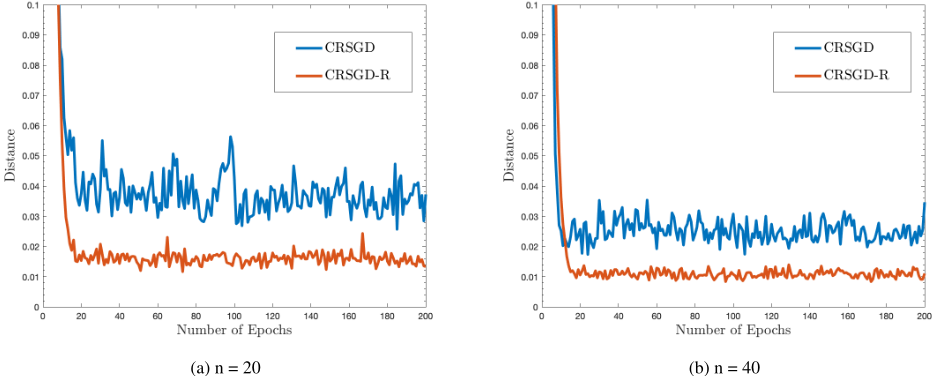
We first demonstrate the experimental results of our centralized distributed algorithm CRSGD-R. We choose the centralized distributed version of Riemannian SGD [Kasai et al., 2018] as the baseline. The number of worker nodes is set to 20 and 40 respectively. The learning rate is set to 0.005 and the batchsize is set to 10. We plot the distance to the optimal solution dist(x, x∗ ) with respect to the number of epochs. The results are shown in Figure 2. According to the experimental results, we can see our CRSGD-R algorithm converges faster than the CRSGD algorithm without random shuffling. The training results of our CRSGD-R algorithm is also more stable than CRSGD. These results validate the effectiveness of random shuffling in centralized distributed Riemannian optimization.
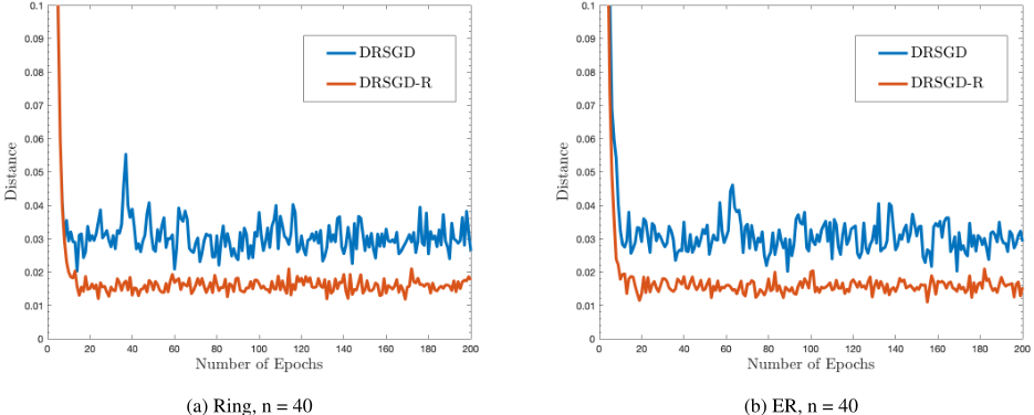
Next we will demonstrate the experimental results of our decentralized distributed algorithm DRSGD-R. We choose decentralized Riemannian SGD [Chen et al., 2021] as the baseline. The decentralized networks considered in the experiment are uniform weighted ring topology and the Erd˝osR´enyi model ER(n, p) associated with the Metropolis constant matrix and the probability p = 0.3. The number of worker nodes is set to 40. Similar to hyperparamter setup of the centralized case, the learning rate is set to 0.005 and the batchsize is set to 10. The stepsize of the consensus step is set to α = 1. We also plot the distance to the optimal solution dist(¯x, x∗ ) with respect to the number of epochs. The results are shown in Figure 1.
According to the experimental results in Figure 1, we can see our DRSGD-R algorithm converges faster than the baseline algorithm DRSGD without random shuffling under different worker node numbers and different topologies. The training results of our RRSGD-R algorithm is also more stable than the baseline algorithm DRSGD. These results verify the effectiveness of random shuffling in decentralized distributed Riemannian optimization.
6 Conclusion
In this paper, we propose the distributed Riemannian stochastic gradient descent algorithms with random shuffling to accelerate the convergence rate of the standard withreplacement SGD algorithm on the Riemannian manifold. We establish the convergence analysis that covers both the conditions of centralized and decentralized learning to improve the SFO complexity of Riemannian SGD from O(ϵ-4 ) to O(√Nϵ-3 ) where N is the size of training data. We conduct the experiment of the leading eigenvector problem under the condition of centralized learning and decentralized learning to validate the performance of our methods.
Acknowledgements
This work was partially supported by NSF IIS 2347592, 2348169, DBI 2405416, CCF 2348306, CNS 2347617, RISE 2536663.
@inproceedings{ijcai2026p566,
  title     = {Accelerated Distributed Riemannian Optimization Algorithms with Random Shuffling},
  author    = {Xian, Wenhan and Huang, Heng},
  booktitle = {Proceedings of the Thirty-Fifth International Joint Conference on
               Artificial Intelligence, {IJCAI-26}},
  publisher = {International Joint Conferences on Artificial Intelligence Organization},
  editor    = {Diego Calvanese},
  pages     = {5083--5091},
  year      = {2026},
  month     = {8},
  note      = {Main Track},
  doi       = {10.24963/ijcai.2026/566},
  url       = {https://doi.org/10.24963/ijcai.2026/566},
}
TY - CPAPER TI - Accelerated Distributed Riemannian Optimization Algorithms with Random Shuffling AU - Xian, Wenhan AU - Huang, Heng T2 - Proceedings of the Thirty-Fifth International Joint Conference on Artificial Intelligence, IJCAI-26 PB - International Joint Conferences on Artificial Intelligence Organization PY - 2026 SP - 5083 EP - 5091 DO - 10.24963/ijcai.2026/566 UR - https://doi.org/10.24963/ijcai.2026/566 ER -Copied
Machine-readable versions of this paper, for tools and AI agents:





