
TransAlpha: Lightweight Design Empowers Stock Return Forecasting
Proceedings of the Thirty-Fifth International Joint Conference on Artificial Intelligence. Main Track. Pages 5209-5217.
https://doi.org/10.24963/ijcai.2026/580
Keywords
- Machine Learning: Supervised Learning
- Machine Learning: Deep learning architectures
- Multidisciplinary Topics and Applications: Finance
- Machine Learning: Applications
Abstract
In intraday stock return forecasting, existing Transformer methods face high computational complexity and do not explicitly handle noisy predictors. We propose TransAlpha, a light-weight Transformer variant tailored for cross section data to advance end-to-end forecasting methods with three novel components (Cross-Sectional Denoising for signal purification, Temporal Attention Gating for trend weighting, and Smart Pooling to avoid information loss) along with a multi-component hybrid loss function. We validate on full A-share market stock data and four key segments (CSI 300/500/1000/2000) with 400 proprietary alpha factors of 15-minute frequencies. TransAlpha outperforms state-of-the-art baselines in predictive power and portfolio profitability, indicating tailored Transformer models have significant practical value in quantitative trade.
- [Bai et al., 2018] Shaojie Bai, J. Zico Kolter, and Vladlen Koltun. An empirical evaluation of generic convolutional and recurrent networks for sequence modeling. In Pro- ceedings of the 35th International Conference on Machine Learning, volume 80, pages 384-393, Stockholm, Swe- den, 2018. PMLR.
- [Bollerslev, 1986] Tim Bollerslev. Generalized autoregres- sive conditional heteroskedasticity. Journal of Economet- rics, 31(3):307-327, 1986.
- [Cao and Tay, 2003] Lijuan Cao and Francis Eng Hock Tay. Support vector machine with adaptive parameters in finan- cial time series forecasting. IEEE transactions on neural networks, 14 6:1506-18, 2003.
- [Chen and Guestrin, 2016] Tianqi Chen and Carlos Guestrin. Xgboost: A scalable tree boosting system. In Proceedings of the 22nd ACM SIGKDD International Conference on Knowledge Discovery and Data Mining, pages 785-794, New York, NY, USA, 2016. ACM.
- [Chung et al., 2014] Junyoung Chung, Caglar Gulcehre, KyungHyun Cho, and Yoshua Bengio. Empirical evalua- tion of gated recurrent neural networks on sequence mod- eling, 2014.
- [Das et al., 2023] Abhimanyu Das, Weihao Kong, Andrew Leach, Shaan K Mathur, Rajat Sen, and Rose Yu. Long- term forecasting with tiDE: Time-series dense encoder. Transactions on Machine Learning Research, 2023. [donghao and wang xue, 2024] Luo donghao and wang xue. ModernTCN: A modern pure convolution structure for general time series analysis. In The Twelfth International Conference on Learning Representations, 2024.
- [Fama, 1970] Eugene F Fama. Efficient capital markets: A review of theory and empirical work. The Journal of Fi- nance, 25(2):383-417, 1970.
- [Gu and Dao, 2024] Albert Gu and Tri Dao. Mamba: Linear- time sequence modeling with selective state spaces. In Proceedings of the 41st International Conference on Ma- chine Learning, volume 235, pages 14890-14904, Vienna, Austria, 2024. PMLR.
- [Hochreiter and Schmidhuber, 1997] Sepp Hochreiter and Jürgen Schmidhuber. Long short-term memory. Neural Computation, 9(8):1735-1780, 1997.
- [Kaplan et al., 2020] Jared Kaplan, Sam McCandlish, Tom Henighan, Tom B Brown, Benjamin Chess, Rewon Child, Scott Gray, Alec Radford, Jeffrey Wu, and Dario Amodei. Scaling laws for neural language models. arXiv preprint arXiv:2001.08361, 2020.
- [Ke et al., 2017] Guolin Ke, Qi Meng, Thomas Finley, Taifeng Wang, Wei Chen, Weidong Ma, Qiwei Ye, and Tie-Yan Liu. Lightgbm: A highly efficient gradient boost- ing decision tree. In Proceedings of the 31st International Conference on Neural Information Processing Systems, volume 30, pages 3146-3154, Red Hook, NY, USA, 2017.
- Curran Associates, Inc. [Li et al., 2023]
- Zhe Li, Shiyi Qi, Yiduo Li, and Zenglin Xu. Revisiting long-term time series forecasting: An investi- gation on linear mapping, 2023.
- [Li et al., 2024] Tong Li, Zhaoyang Liu, Yanyan Shen, Xue Wang, Haokun Chen, and Sen Huang. Master: Market- guided stock transformer for stock price forecasting. In Proceedings of the Thirty-Eighth AAAI Conference on Ar- tificial Intelligence and Thirty-Sixth Conference on In- novative Applications of Artificial Intelligence and Four- teenth Symposium on Educational Advances in Artificial Intelligence, AAAI'24/IAAI'24/EAAI'24, New York, NY, USA, 2024. AAAI Press.
- [Liu et al., 2022] Shizhan Liu, Hang Yu, Cong Liao, Jian- guo Li, Weiyao Lin, Alex X. Liu, and Schahram Dust- dar. Pyraformer: Low-complexity pyramidal attention for long-range time series modeling and forecasting. In Inter- national Conference on Learning Representations, 2022.
- [Liu et al., 2024] Yong Liu, Tengge Hu, Haoran Zhang, Haixu Wu, Shiyu Wang, Lintao Ma, and Mingsheng Long. itransformer: Inverted transformers are effective for time series forecasting, 2024.
- [Nie et al., 2023] Yuqi Nie, Nam H. Nguyen, Phanwadee Sinthong, and Jayant Kalagnanam. A time series is worth 64 words: Long-term forecasting with transformers. In International Conference on Learning Representations, 2023.
- [Park et al., 2025] Kijeong Park, Sungchul Hong, and Jong- June Jeon. Dynamic higher-order relations and event- driven temporal modeling for stock price forecasting. In Proceedings of the 34th International Joint Conference on Artificial Intelligence (IJCAI), 2025.
- [Salinas et al., 2020] David Salinas, Valentin Flunkert, and Jan Gasthaus. Deepar: Probabilistic forecasting with au- toregressive recurrent networks. International Journal of Forecasting, 36(3):1181-1191, 2020.
- [Shi et al., 2025] Xiaoming Shi, Shiyu Wang, Yuqi Nie, Di- anqi Li, Zhou Ye, Qingsong Wen, and Ming Jin. Time- moe: Billion-scale time series foundation models with mixture of experts. In International Conference on Learn- ing Representations (ICLR), 2025.
- [Vaswani et al., 2017] Ashish Vaswani, Noam Shazeer, Niki Parmar, Jakob Uszkoreit, Llion Jones, Aidan N Gomez, Łukasz Kaiser, and Illia Polosukhin. Attention is all you need. In Advances in Neural Information Processing Sys- tems, volume 30, pages 5998-6008, Red Hook, NY, USA, 2017.
- [Curran Associates, Inc. Wu et al., 2021] Haixu Wu, Jiehui Xu, Jianmin Wang, and Mingsheng Long. Autoformer: Decomposition transform- ers with Auto-Correlation for long-term series forecasting. In Advances in Neural Information Processing Systems, volume 34, pages 22083-22094, Red Hook, NY, USA, 2021.
- [Curran Associates, Inc. Wu et al., 2022] Haixu Wu, Tengge Hu, Jianmin Wang, Mingsheng Long, Qing Wang, Jian Pei, Tong Yu, and Chuxu Zhang. Timesnet: Temporal 2d-variation model- ing for general time series analysis. In Proceedings of the 39th International Conference on Machine Learning, pages 23008-23020, Baltimore, MD, USA, 2022. PMLR.
- [Yu et al., 2024] Zhaojian Yu, Yinghao Wu, Genesis Wang, and Heming Weng. Miga: Mixture-of-experts with group aggregation for stock market prediction, 2024.
- [Zeng et al., 2023] Ailing Zeng, Muxi Chen, Lei Zhang, and Qiang Xu. Are transformers effective for time series fore- casting? In Proceedings of the Thirty-Seventh AAAI Con- ference on Artificial Intelligence and Thirty-Fifth Confer- ence on Innovative Applications of Artificial Intelligence and Thirteenth Symposium on Educational Advances in Artificial Intelligence, AAAI'23/IAAI'23/EAAI'23. AAAI Press, 2023.
- [Zhang and Yan, 2023] Yunhao Zhang and Junchi Yan. Crossformer: Transformer utilizing cross-dimension de- pendency for multivariate time series forecasting. In The Eleventh International Conference on Learning Represen- tations, 2023.
- [Zhang et al., 2024] Xiyuan Zhang, Ranak Roy Chowdhury, Rajesh K. Gupta, and Jingbo Shang. Large language mod- els for time series: a survey. In Proceedings of the Thirty- Third International Joint Conference on Artificial Intelli- gence, IJCAI '24, 2024. IJCAI
- [Zhou et al., 2021] Haoyi Zhou, Shanghang Zhang, Jieqi Peng, Shuai Zhang, Jianxin Li, Hui Xiong, and Wancai Zhang. Informer: Beyond efficient transformer for long sequence time-series forecasting. In Proceedings of the 38th International Conference on Machine Learning, vol- ume 139, pages 11106-11116, Online, 2021. PMLR.
- [Zhou et al., 2022] Tian Zhou, Ziqing Ma, Qingsong Wen, Xue Wang, Liang Sun, and Rong Jin. Fedformer: Fre- quency enhanced decomposed transformer for long-term series forecasting, 2022.
- [Zhu et al., 2024] Peng Zhu, Yuante Li, Yifan Hu, Qinyuan Liu, Dawei Cheng, and Yuqi Liang. Lsr-igru: Stock trend prediction based on long short-term relationships and im- proved gru. In Proceedings of the 33rd ACM International Conference on Information and Knowledge Management, CIKM '24, page 5135-5142, New York, NY, USA, 2024. Association for Computing Machinery.
- [Zou et al., 2023] Jinan Zou, Qingying Zhao, Yang Jiao, Haiyao Cao, Yanxi Liu, Qingsen Yan, Ehsan Abbasnejad, Lingqiao Liu, and Javen Qinfeng Shi. Stock market pre- diction via deep learning techniques: A survey, 2023.
References were extracted automatically from the PDF and may contain errors.
Full text extracted automatically from the PDF; figures, tables and equations may differ. The PDF is the version of record.
1 Introduction
Stock return forecasting has advanced with AI. A solid forecasting method and stable prediction results can impact portfolio optimization and trading strategies. Practical stock forecasting methods can be categorized into time series forecasting models that use temporal sequences of individual stocks and multi-factor models that learn universal factor-return relationships across stocks and time via cross-sectional data. In recent years, Transformer [Vaswani et al., 2017] approaches rise as an alternative for time series forecasting. Despite their success in processing language tokens, Transformers fail to replicate breakthroughs in time series forecasting. Influential work such as DLinear [Zeng et al., 2023] is skeptical about whether complex Transformer architectures can outperform linear models. In particular, stock forecasting fundamentally differs from other time series forecasting tasks in the following aspects of challenges: (1) Weak signal-to-noise ratio: predictive features (alpha) signals are subtle, prune to noise and overfitting [Fama, 1970]. Signals are diluted if model has multiple compositions and residual connection blocks, which can decrease predictive power; (2) High dimensionality of cross-sectional data: quantitative trading strategies contain hundreds of alpha factors, introducing inter-dependencies [Li et al., 2024]; (3) Non-stationarity and volatility: market micro-structures shift rapidly; trained models cannot generalize across time. As a result, leading quantitative companies still rely on more robust and interpretable linear models to combine with existing trading strategies for stable profit, but invest heavily in Transformer and Large Language Model (LLM) research to explore possibilities improving model's predictive power.
Our work comes from a realistic production environment of a quantitative company: we demonstrate Transformer model theories can be transferred to a profitable pipeline using proprietary alpha factors in A-Share market. We propose TransAlpha, a lightweight transformer-based architecture for stock return forecasting. Our main contributions are three-fold:
- A systematic investigation that incorporates state-ofthe-art time series model architectures into multi-factor framework to examine their effectiveness for stock return forecasting.
- A domain-tailored Transformer architecture with three novel components: cross-sectional denoising, temporal attention gating, and smart pooling, all validated by real trading data.
- An industry-aligned pipeline that enables for training and back-testing custom models under a realistic setup with custom strategies.
These components address universal challenges such as noise in high-dimensional data, inefficient attention, and information loss when pooling. We balance academic reproducibility and proprietary privacy by providing the processed data files with anonymous alpha factors.
The remainder of this paper is organized as follows: Section 2 reviews related work in time series forecasting methods and past stock forecasting attempts. Section 3 presents the TransAlpha architecture. Section 4 presents research questions and experimental results. Section 5 concludes.
2 RelatedWork
2.1 Times Series Forecasting
Traditional time series methods are maximum likelihoodbased statistical models, such as ARIMA, and GARCH [Bollerslev, 1986]. Both methods and their variants assume stationarity, which are usually unrealistic, especially in intraday price movements. Later, a shift to machine learning introduced tree-based models such as XGBoost [Chen and Guestrin, 2016], LightGBM [Ke et al., 2017]. They can capture non-linearity without distribution or stationarity assumptions. Further, LSTMs [Hochreiter and Schmidhuber, 1997] addressed the vanishing gradient problem, and DeepAR [Salinas et al., 2020] pioneered in probabilistic forecasting. In addition, Convolutional Neural Network (CNN) models such as TCN [Bai et al., 2018] and TimesNet [Wu et al., 2022] use convolutional layers to capture local temporal patterns. Modern TCN [donghao and wang xue, 2024] refines TCN with much larger effective receptive fields. Later, Transformer [Vaswani et al., 2017] replaced LSTM's recurrent layers with self-attention, enabling long-range dependency modeling. Transformer adaptations for time series faced high computational complexity up to O(L2 ), where L is sequence length. Many variants are introduced to tackle this issue and attempt novel structures to solve long-sequence forecasting problem. Informer [Zhou et al., 2021] proposes probability sparse attention to approximate the full attention matrix. Autoformer [Wu et al., 2021] decomposes series to trend and seasonal components. PatchTST [Nie et al., 2023] frames time series as tokens. Pyraformer [Liu et al., 2022] proposes pyramidal attention to hierarchically compress temporal information. Crossformer [Zhang and Yan, 2023] establishes a Hierarchical Encoder-Decoder (HED) to use the information at different scales; iTransformer [Liu et al., 2024] simply applies the attention and feed-forward network on the inverted dimensions. New direction involves adapting LLM techniques [Zhang et al., 2024]. Time-MoE [Shi et al., 2025] used a sparse Mixture-of-Experts (MoE) design based on scaling laws [Kaplan et al., 2020] with 2.4 billion parameters but only activate a subset of experts.
2.2 Stock Return Prediction
The fluctuation of stock prices is influenced by a complex array of factors. Therefore, there is a need to utilize machine learning techniques [Zou et al., 2023]. Models must balance between predictive power and noise robustness. Successful adaptations can date back to support vector machines (SVMs) methods [Cao and Tay, 2003]. LSTMs and GRUs [Zhu et al., 2024] were also adapted. Graph WaveNet, [Park et al., 2025]) incorporates Graph Neural Networks (GNNs) and hypergraphs to capture higher-order stock relationships. Mamba [Gu and Dao, 2024] integrates selective State-Space models (SSMs) into a simplified end-to-end neural network architecture. MASTER [Li et al., 2024] introduced marketguided attention to prioritize macroeconomic signals over price fluctuations; MIGA [Yu et al., 2024] employed a MoE framework to partition experts by temporal frequency. Despite these advances, several gaps remain in the literature: (1) few works validate their models on high-dimensional alpha data from real production environment; (2) there are limited studies systematically studying performance of Transformer models in stock forecasting. (3) successful methods and insights are typically non-disclosed for proprietary concerns.
3 Methodology
3.1 ProblemFormulation
We formalize stock return forecasting as a supervised learning task. Let S = {s1, s2, . . . , sN} denote the A-share stock universe, where N represents the total number of stocks. Let T denote the set of 15-minute cross sections within the observation period. For each cross section t ∈ T, the alpha factor matrix at time t is denoted as Xt ∈ RN×D , where D = 400 is the dimension of alpha factors, and each row xt,s ∈ RD corresponds to the factor value vector of stock s at time t. The true return vector at time t is Yt ∈ RN , where each element yt,s represents the 15-minute forward raw return of stock s at time t.
We use a look-back window of fixed length L = 16, corresponding to 16 consecutive 15-minute cross sections. Then, we construct a sequence of factor matrices {Xt-L+1,Xt-L+2, . . . ,Xt}, where each matrix inside describes the cross-sectional distribution of factor values across all stocks at a t. The forecasting model maps this temporal sequence of cross-sectional factor data to a predicted return vector ˆYt+1 ∈ RN for the next 15-minute cross section:
where f denotes the model, and Θ is the set of trainable parameters. The observation period T is partitioned into nonoverlapping subsets of train, validation, and test segments.
3.2 Model
We propose TransAlpha for intraday cross-sectional stock return forecasting in the A-share market. The model addresses three challenges: (1) idiosyncratic noise in alpha factor signals, (2) time-step relevance heterogeneity in intraday trends, and (3) signal dilution induced by over-engineering. We formalize the model following section 3.1.
Let X = {Xt-L+1,Xt-L+2, . . . ,Xt} denote the input to TransAlpha. X is a temporal sequence of cross-sectional alpha factor matrices, where X ∈ RN×D . The output is a predicted 15-minute forward return vector ˆYt+1 ∈ RN . To present the three core modules of the model, we define the intermediate variables first. Let Xdenoise ∈ RN×L×D be the denoised factor, Z ∈ RN×L×d be the projected feature, and Zgated ∈ RN×L×d be the time-weighted feature, where d is the model's hidden dimension. We use d = 64 for all baseline models. Let Zpool ∈ RN×2d denote the aggregated features, and we define an output head that maps the aggregated features to predicted returns. The end-to-end workflow is demonstrated in Figure 1
Cross-Sectional Denoising The Cross-Section Denoising (CSD) module separates stock-specific alpha signals from market-wide systematic beta signals, with adaptive scaling to suppress noise while preserving predictive components. For an input X ∈ RN×L×D , let β be the market-wide signal, and α be the stock-specific residual. They are defined and obtained by

where β ∈ R1×L×D and α ∈ RN×L×D . We introduce a fixed scalar hyperparameter τ = 10-3 to partition the stockspecific alpha signal into noisy alphas (|α| ≤ τ) and nonnoisy, predictive alphas (|α| > τ). Further, let sα, sβ ∈ R1×1×D be factor-wise trainable scaling tensors. sα is applied exclusively to the non-noisy components α. During training, sα is optimized to amplify factors with high predictive power and dampen factors with weak signals, without affecting noisy components. Similarly, sβ is applied uniformly to the market-wide systematic signal β. Training optimizes sβ to down-weight overly dominant systematic trends and upweight stable, predictive market signals, ensuring a balanced combination of idiosyncratic and systematic components for return forecasting. We then combine both components and obtain the denoised input:
where 1(·) is the indicator function and ⊙ denotes elementwise multiplication.
Temporal Attention Gating The Temporal Attention Gating (TAG) module uses relevance to return predictions to weight time steps so that model can capture intraday trend with minimal complexity. The denoised sequence Xdenoise is projected to model dimension d to yield Z via a feed-forward block.
where Linear(X) =WX+ b is a linear layer with trainable parameters W, b. We then transformed Z to Zgated = Z⊙wt. The attention time-step weights wt are computed as
where wt sums to 1 to ensure signal weights are normalized. TAG performs element-wise multiplication of attention weights with the entire temporal sequence to generate Zgated, while traditional approaches only applies gating to the final hidden state. Meanwhile, TAG replaces the complex multi-head attention with a single-head scalar-scoring attention layer and removes positional encoding for further simplification.
Smart Pooling and Output Head The Smart Pooling (SP) component aggregates time-weighted features into fixeddimensional vectors by combining the most recent time step and max pooled peak signals with extreme volatility. Let Zgated ∈ RN×L×d be output from TAG module, we define Zlast as the most recent time step, Zmax as the max-pooled feature, and Zpool as the concatenated features, and denote
ˆYt+1 as the predicted returns. We present Zlast and Zmax using standard tensor indexing, where the first dimension is individual stocks, second dimension is intraday time steps and third dimension is model's hidden feature.
where MLP denotes a two-layer perceptron, and Concat[· , · ] denotes feature concatenation along the last dimension. The pooling used direct concatenation instead of average or sum in traditional pooling methods that lead to information loss.
3.3 Training
We design a multi-component loss function specifically adapted to intraday cross-sectional stock return forecasting. The loss is designed to balance regression performance, linear correlations between predicted and actual returns, relative rank accuracy, and regularization to penalize parameter size.
where λ1, . . . , λ5 are non-negative weighting coefficients. Let ˆYt+1 = {ˆ yt+1,s}s∈S and Yt+1 = {yt+1,s}s∈S be the vectors of predicted and true forward returns for time t + 1, respectively, and ¯ˆ yt+1, ¯ yt+1 be their cross-sectional means. We elaborate on each loss component as follows. First, the quantile ranking loss Lrank penalizes misalignment between predicted and true rankings of top and bottom stocks by enforcing a minimum predicted return gap between the top 20% and bottom 20% of stocks, sorted by true returns, with a margin m = 0.1, formulated as:
where ˆ ytop t+1,s and ˆ ybottom t+1,s are predicted returns for top/bottom quantile stocks, and E[·] denotes the expectation over training samples. Next, the Huber loss Lhuber robustifies training against extreme returns by balancing mean squared error (MSE) for small prediction errors and mean absolute error (MAE) for outliers. Let ϵt+1,s = ˆ yt+1,s - yt+1,s denote the prediction error for stock s, the loss with threshold δ = 1.0 is:
The correlation loss term Lcorr minimizes 1 - ρpearson, where ρpearson is the pearson correlation coefficient. We denote auxiliary terms for cross-covariance and the product of standard deviations:
such that Lcorr = 1 - Ccov/Cstd. The product correlation loss Lprod jointly maximize both correlations. Given a crosssectional vector of values V = {vs}s∈S, the rank operator maps V to a rank vector by rank(V) = {rs}s∈S , where rs is the ordinal rank of vs in V (1 smallest, N largest). The operator converts continuous return values into ordinal ranks. Consequently, ρpearson = Ccov/Cstd and
Then, the product loss is Lprod = 1 - ρpearson · ρspearman.
Finally, the regularization loss Lreg = λreg∥θ∥22 (with λreg = 10-5 ) prevents overfitting to training data noise, where ∥ · ∥2 denotes the ℓ2 norm. The weighting coefficients for the total loss function are chosen to prioritize ranking and correlation objectives. We set small weights for huber and regularization components. The final utilized weights are determined empirically: λ1 = 0.4, λ2 = 0.05, λ3 = 0.4, λ4 = 0.1, λ5 = 0.05.
3.4 Inference
After obtaining the trained model, we map the test file's crosssectional sequence, with input batch size B, to return predictions in the next time period. For each cross section t, we maintain a sliding look-back window of length L and apply two preliminary filters before feeding the batch.
Look-back Completeness Filter The completeness filter discards sequences which do not contain enough valid time steps (< L) in a look-back window. Formally, the filter retains only sequences satisfying:
where ∅ represent an empty factor matrix without valid stocks at time τ.
NaNElimination Filter For each time step τ in a complete look-back window, the NaN elimination filter removes rows with missing or non-finite factor values, typically caused by trading halts or data feed errors. Let Xτ (i, j) denote the j-th factor value of the i-th stock at time τ. The cleaned crosssectional matrix ˜Xτ ∈ R ˜Nt×D , where ˜Nt ≤ Nt is the number of valid stocks at time τ) is defined as,
where Xτ(i, :) denotes the i-th row of Xτ , and Rfin = R \ {NaN,±∞} denotes the set of finite real numbers. The filter ensures all elements of ˜Xτ are valid real numbers, maintaining numerical stability of forward pass. The filtered sequence ˜Xt = { ˜Xt-L+1, . . . , ˜Xt} is then reshaped into a
Algorithm 1 TransAlpha Forward Pass
- 1: Step 1: Cross-Sectional Denoising
- 2: β = 1B ∑Bi=1 Xi ∈ R1×L×D
- 3: α =X-β ∈ RB×L×D
- 4: αscaled = α(sα ⊙1(|α| > τ) +1(|α| ≤ τ))
- 5: βscaled = β ⊙ sβ
- 6: Xdenoise = αscaled +βscaled ∈ RB×L×D
- 7: Step 2: Input Projection toModel Dimension
- 8: Z1 = Linear(Xdenoise) ∈ RB×L×dmodel
- 9: Z2 = LayerNorm(Z1) ∈ RB×L×dmodel
- 10: Z3 = ReLU(Z2) ∈ RB×L×dmodel
- 11: Step 3: Temporal Attention Gating
- 12: wt = Softmax(Linear(Z3)) ∈ RB×L×1
- 13: Zgated = Z3 ⊙wt ∈ RB×L×dmodel
- 14: Step 4: Smart Temporal Pooling
- 15: Zlast = Zgated[:,-1, :] ∈ RB×dmodel
- 16: Zmax =maxLt=1 Zgated[:, t, :] ∈ RB×dmodel
- 17: Zpool = Concat(Zlast,Zmax) ∈ RB×2dmodel
- 18: Step 5: Output Head
- 19: ˆY =MLP(Zpool) ∈ RB×1
- 20: Return: ˆY
three-dimensional tensor X compatible with the TransAlpha model input size, which is then feeded into the forward pass workflow in Algorithm 1.
3.5 Convergence Analysis
For simplicity, we sketch TransAlpha's convergence to the true return Yt+1 under three mild assumptions. (1) Multicomponent loss L is Lipschitz continuous. (2) Model parameters (sα, sβ,W) are bounded via Lreg in a compact parameter space Θ. (3) Training uses mini-batch Adamwith decreasing learning rate ηk ∝ 1/√k. The expected loss satisfies
where C > 0 is a constant, Θ∗ is optimal parameter. As epochs k → ∞, ∥ ˆYt+1(Θk) - Yt+1∥2 → 0.
3.6 Complexity Analysis
Let h be the number of attention heads in baseline models, K be TCN kernel size, G be crossformer's segment size. TransAlpha's time complexity is derived by calculating floatpoint operations. The input projection is the dominant term.
where TCSD is CSD's mean aggregation and element-wise operations on input tensors, TProj is input projection's linear mapping of D-dimensional alpha factors to d-dimensional model features. TTAG is TAG's linear layer and element-wise gating on N × L × d features, and TMLP is the output MLP's time complexity which contains two linear layers operated on 2d-dimensional pooled features. Table 1 summaries the time complexity of TransAlpha and baseline models.
| Model | Time Complexity | Space Complexity |
|---|---|---|
| TransAlpha | O(NLDd) | O(NLDd) |
| DLinear | O(NLDd) | O(NLDd) |
| TCN | O(NLdK) | O(NLDd) |
| Informer | O(NLd logL) | O(NLDd) |
| Autoformer | O(NLd) | O(NLDd) |
| Pyraformer | O(NLd logL) | O(NLDd) |
| Crossformer | O(NLdL/G) | O(NLDd) |
| iTransformer | O(NL2 d/h) | O(NLDd) |
TransAlpha's space complexity is dominated by intermediate activation tensors (N × L × d), resulting in an asymptotic complexity of O(NLd), identical to all baseline models. Trainable parameters O(Dd+d2 ) are negligible in comparison to activation memory usage. In terms of time efficiency, TransAlpha ranks the best, highlighting its lightweight characteristic. Autoformer has the same nominal O(NLd) time complexity, but its practical efficiency is lower due to Fast Fourier Transform (FFT) during decomposition. Crossformer introduces an extra L/G overhead factor. Informer and Pyraformer add a logL factor. iTransformer introduces an L2 /h factor, and TCN adds a kernel size factor K.
4 Experiments
We formulate three core research questions (RQs).
- RQ1: Are Transformer models effective in general? How is TransAlpha's predictive power across different market segments?
- RQ2: Can the models transfer their predictive power into profit in back-test?
- RQ3: Are the proposed architectures effective?
- RQ4: Do TransAlpha's prediction patterns exhibit distinct characteristics?
4.1 Experimental Set up
Data Set Details We evaluate on an intraday dataset directly coming from production environment, covering the entire A-share market (Shanghai and Shenzhen Stock Exchanges), with four key market segments (CSI 300, CSI 500, CSI 1000, and CSI 2000) for subset modeling to assess generalization ability across market capitalization. The dataset contains 400 proprietary alpha factors in 15-minute frequency cross-sectionals stored in HDF5 format and are normalized without extreme values. The observation period is non-overlapping, consisted of training (2021-01-04 to 202309-28), validation (2023-10-09 to 2023-12-29), and testing (2024-01-02 to 2024-12-31) sets to avoid look-ahead bias and ensure out-of-sample evaluation. There are Nd = 242 trade days, each from 09:45 am to 15:00 pm daily (Nt = 16 cross sections per day, total of T = Nd ×Nt = 3856). Transaction costs are applied only on position liquidation at 0.1% per trade, inclusive of fees.
Baseline Models We compare TransAlpha against 3 categories of baselines. Linear models include DLinear [Zeng et al., 2023], RLinear [Li et al., 2023], and TiDE [Das et al., 2023]. Non-Transformer DL models include GRU [Chung et al., 2014], DeepAR [Salinas et al., 2020], and TCN [Bai et al., 2018], TimesNet [Wu et al., 2022], Modern TCN [donghao and wang xue, 2024]. Transformer models include Informer [Zhou et al., 2021], Autoformer [Wu et al., 2021], PatchTST [Nie et al., 2023], Pyraformer [Liu et al., 2022], Crossformer [Zhang and Yan, 2023], Fedformer [Zhou et al., 2022] and iTransformer [Liu et al., 2024].
Implementation Details Our model is implemented in PyTorch 2.7.0 with CUDA11.8. All experiments are conducted on a server equipped with an AMD EPYC 7T83 64-Core Processor (256 total CPUs across 2 NUMA nodes, 64 physical cores per socket, 128 siblings per node) and 1.5 TiB system memory. For training, we utilized a cluster of four NVIDIA GeForce RTX 4090 GPUs (24564 MiB VRAM per GPU). We use grid search to perform hyperparameter optimization and obtain optimal values based on validation set. We trained the model separately for all market subsets and adopted a naive long-short 50 strategy to back-test.
Evaluation Metrics Stock price forecasting's success is measured by trading profitability rather than point prediction accuracy. Traditional forecasting metrics such as MSE fail to capture the relative performance rankings that drive quant trading strategies. We use the Information Coefficient (IC), Rank IC, Information Coefficient Information Ratio (ICIR) and Rank ICIR to quantify predictive power. We evaluate a model's profitability power using the Annualized Return (AR), Information Ratio (IR), Sharp Ratio (SR), Maximum Drawdown (MDD) and Turn over Rate (TR).
4.2 RQ1Model Predictive Power
We experiment on both the full market data and all CSI indices subsets to evaluate TransAlpha's predictive power under different market segments, via these standard metrics. See Table 3's first four columns. Overall, TransAlpha's predictive power is consistent across all subsets and constantly among the top models. Notably, subsets with more stocks do not always mean performance increase.
4.3 RQ2 Backtest Result
Overall, TransAlpha offers strong AR, IR and SR, with notable lead in SR. Most importantly, strong predictive power does not necessarily transfer to profitability, a sign of overfitting, with iTransformer as a typical example. MDD < 0.05 suggests worst peak-to-trough loss is less than 5% at any point. TR < 0.20 suggests it only needs to rebalance the portfolio by less than 20% regularly, consuming low trading costs and minimal operational hassle. TransAlpha maintains all lower than the empirical thresholds, offering stable predictions.
| Model | Subset | IC | Rank IC | ICIR | Rank ICIR | AR | IR | SR | MDD | TR |
|---|---|---|---|---|---|---|---|---|---|---|
| No CSD | CSI 300 CSI 500 CSI 1000 CSI 2000 Full Market | 0.0594 (0.1583) ↓ 0.0671 (0.1582) ↓ 0.0966 (0.1271) 0.1412 (0.0958) 0.1430 (0.0825) | 0.0726 (0.1673) 0.0704 (0.1569) 0.0727 (0.1504) ↓ 0.1029 (0.1130) ↓ 0.0972 (0.1251) | 0.3755 (2.6629) ↓ 0.4240 (2.3583) ↓ 0.7598 (1.3161) 1.4745 (0.6782) 1.7331 (0.5770) | 0.4340 (2.3042) ↓ 0.4487 (2.2288) ↓ 0.4835 (2.0682) ↓ 0.9110 (1.0977) 0.7769 (1.2872) | 0.2761 (0.0997) 0.2785 (0.0953) 0.2733 (0.1033) 0.4861 (0.0717) 0.4333 (0.1095) | 3.1715 (0.0879) ↓ ↓ 3.0832 (0.0731) ↓ ↓ 3.0285 (0.0885) ↓ ↓ 7.7130 (0.0879) ↓ 4.1331 (0.0797) | 2.8670 (0.0843) 2.8317 (0.0730) 2.7356 (0.0847) 7.2162 (0.0857) 3.9085 (0.0798) | ↓ 0.0550 ↓ ↓ 0.0548 ↓ ↓ 0.0594 ↓ 0.0202 0.0918 ↓ | 0.2105 ↓ 0.2090 ↓ 0.2142 ↓ 0.2447 ↓ 0.2557 ↓ |
| No TAG | CSI 300 CSI 500 CSI 1000 CSI 2000 Full Market | 0.0604 (0.1619) ↓ 0.0671 (0.1582) ↓ 0.0966 (0.1271) 0.1407 (0.0962) ↓ 0.1406 (0.0834) | 0.0730 (0.1707) 0.0704 (0.1567) 0.0726 (0.1500) ↓ 0.1022 (0.1123) ↓ 0.0941 (0.1210) ↓ | 0.3730 (2.6813) ↓ 0.4246 (2.3552) ↓ 0.7597 (1.3163) 1.4625 (0.6838) ↓ 1.6856 (0.5933) | 0.4275 (2.3390) ↓ 0.4495 (2.2249) ↓ 0.4842 (2.0654) ↓ 0.9102 (1.0986) 0.7782 (1.2851) | 0.2710 (0.0939) ↓ 0.2795 (0.1001) ↓ 0.2729 (0.0969) ↓ 0.4780 (0.0693) ↓ 0.3851 (0.1058) ↓ | 2.9056 (0.0653) ↓ 3.1722 (0.0873) ↓ 2.9461 (0.0716) ↓ 7.5524 (0.0804) 3.8507 (0.0796) ↓ | 2.6877 (0.0661) 2.8746 (0.0834) 2.7063 (0.0718) 7.1118 (0.0798) 3.6110 (0.0814) | ↓ 0.0623 ↓ ↓ 0.0548 ↓ ↓ 0.0594 ↓ 0.0202 ↓ 0.0877 ↓ | 0.1909 0.2093 ↓ 0.2163 ↓ 0.2472 ↓ 0.2507 ↓ |
5 Conclusions
This paper tackles challenges of forecasting noisy crosssection data in a real stock market context. We introduce TransAlpha, a lightweight Transformer variant. Extensive experiments suggest it outperforms on core trading metrics and its core components are effective to handle noise. Beyond finance, CSD has the potential to denoise sensor data in manufacturing; TAG can prioritize time steps in patient monitoring; Smart Pooling can aggregate sparse signals in traffic flow. The experiments are exclusively conducted on A-Share market, using proprietary alpha factors from a single quantitative firm. Also, TransAlpha relies on a fixed lookback window and static loss function weights. In future work, we will extend to American stock markets and include MoE components with tailored experts to scale up parameter size, incorporating methods to adapt dynamic market conditions. Finally, we will test the architecture in different forecasting tasks, such as the benchmark data sets in long-range time series forecasting.
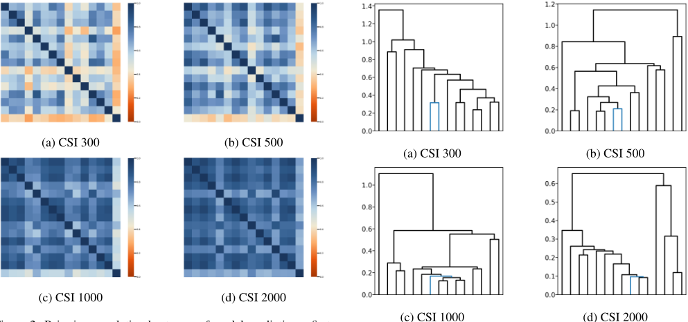
Figure 2: Pairwise correlation heatmaps of model predictions: first row and column are TransAlpha, with the rest models sorted in alphabetical order.
4.4 RQ3 Ablation Study
We include an ablation study to test the effectiveness of core components in TransAlpha by removing CSD and TAG portion respectively. Table 2 shows an evident drop in backtest metrics especially IR and SR after removing either core components, which indicates the components are effective in boosting profitability. Specifically, CSD can reduce the over-fitting issue, which can be generalized to other highdimensional forecasting tasks. TAG also verifies its efficiency gain over standard multi-head attention O(NLD) vs O(NL2D).
4.5 RQ4 Pattern distinction
The model's generated predictions offer distinct patterns from heatmaps and dendrograms of hierarchical clustering. See Figure 2, 3. On large-cap subsets (CSI 300 and CSI 500), the correlations are much lower, indicating the model learned distinct pattern compared to other baselines.
| Model | Subset | IC | Rank IC | ICIR | Rank ICIR | AR | IR | SR | MDD | TR |
|---|---|---|---|---|---|---|---|---|---|---|
| DLinear | CSI 300 | 0.0594 (0.1654) 0.0734 (0.1718) | 0.3589 (2.7867) | 0.4271 (2.3414) | 0.2806 (0.0946) | 3.4093 (0.0866) | 3.0843 (0.0832) | 0.0414 | 0.2144 | |
| CSI 500 | 0.0553 (0.1623) | 0.0639 (0.1659) | 0.3408 (2.9347) | 0.3851 (2.5966) | 0.2505 (0.0904) | 2.8461 (0.0686) | 2.6050 (0.0689) | 0.0396 | 0.2000 | |
| CSI 1000 CSI 2000 | 0.0709 (0.1581) 0.1090 (0.0996) | 0.0749 (0.1828) 0.1021 (0.1080) | 0.4483 (2.2306) 1.0942 (0.9139) | 0.4099 (2.4399) 0.9459 (1.0572) | 0.3191 (0.1253) 0.4938 (0.0650) | 2.9161 (0.0906) 8.0408 (0.0761) | 2.6640 (0.0862) 7.6304 (0.0756) | 0.0677 0.0222 | 0.1995 0.2407 | |
| Full Market | 0.0968 (0.0890) | 0.0909 (0.1079) | 1.0879 (0.9192) | 0.8419 (1.1878) | 0.4883 (0.0731) | 6.8408 (0.0694) | 6.5296 (0.0697) | 0.0286 | 0.2461 | |
| RLinear | CSI 300 | 0.0558 (0.1486) | 0.0662 (0.1546) | 0.3757 (2.6618) | 0.4282 (2.3353) | 0.2258 (0.0852) 0.2343 (0.0821) | 2.9396 (0.0804) 3.2582 (0.0862) | 2.6264 (0.0784) 2.9063 (0.0823) | 0.0454 0.0326 | 0.2174 0.2510 |
| CSI 500 CSI 1000 | 0.0561 (0.1467) 0.0713 (0.1245) | 0.0628 (0.1409) 0.0633 (0.1279) 0.1031 (0.1326) | 0.3825 (2.6141) 0.5724 (1.7471) | 0.4453 (2.2455) 0.4948 (2.0209) | 0.2297 (0.0801) | 3.1378 (0.0794) 5.7123 (0.0761) | 2.8153 (0.0795) 5.4123 (0.0760) | 0.0374 0.0562 | 0.2364 | |
| CSI 2000 Full Market | 0.1084 (0.1141) 0.1000 (0.0890) | 0.0880 (0.1066) | 0.9496 (1.0531) 1.1238 (0.8899) | 0.7777 (1.2859) 0.8257 (1.2110) | 0.4856 (0.0903) 0.4254 (0.0751) | 5.9529 (0.0748) | 5.6182 (0.0766) | 0.0363 | 0.1986 0.2472 | |
| TiDE | CSI 300 | 0.0524 (0.1696) | 0.0679 (0.1699) | 0.3090 (3.2360) | 0.3997 (2.5018) | 0.2506 (0.0994) | 2.8438 (0.0843) | 2.5575 (0.0808) | 0.0625 | 0.1958 |
| CSI 500 CSI 1000 | 0.0558 (0.1339) 0.0953 (0.1203) | 0.0548 (0.1196) 0.0686 (0.1367) | 0.4170 (2.3981) 0.7923 (1.2622) | 0.4579 (2.1840) 0.5017 (1.9932) | 0.2133 (0.0694) 0.2403 (0.0816) | 3.2947 (0.0761) 2.9880 (0.0675) | 2.9460 (0.0749) 2.7312 (0.0679) | 0.0333 0.0507 | 0.2326 0.2395 | |
| CSI 2000 | 0.1352 (0.0972) 0.1334 (0.0896) | 0.1029 (0.1148) | 1.3904 (0.7192) | 0.8964 (1.1155) | 0.4766 (0.0659) | 7.3414 (0.0699) | 7.0129 (0.0708) | 0.0261 | 0.2438 | |
| Full Market | 0.0945 (0.1206) | 1.4891 (0.6715) | 0.7835 (1.2764) | 0.3956 (0.0862) | 4.8776 (0.0779) | 4.5766 (0.0779) | 0.0515 | 0.2650 | ||
| GRU | CSI 300 | 0.0509 (0.1472) | 0.0579 (0.1460) | 0.3460 (2.8900) | 0.3963 (2.5231) | 0.1624 (0.0731) | 2.3928 (0.0762) | 2.0680 (0.0742) | 0.0494 | 0.2124 |
| CSI 500 | 0.0467 (0.1130) | 0.0437 (0.0889) | 0.4134 (2.4188) | 0.4916 (2.0342) | 0.0990 (0.0468) | 2.3152 (0.0785) | 1.8153 (0.0782) | 0.0184 | 0.2215 | |
| CSI 1000 CSI 2000 | 0.0945 (0.1197) 0.1324 (0.1032) | 0.0681 (0.1312) 0.1043 (0.1158) | 0.7897 (1.2663) 1.2834 (0.7792) | 0.5188 (1.9274) 0.9006 (1.1104) | 0.2413 (0.0890) 0.4941 (0.0742) | 2.9601 (0.0793) 7.0501 (0.0753) | 2.6689 (0.0780) 6.6904 (0.0740) | 0.0535 0.0270 | 0.2186 | |
| Full Market | 0.1366 (0.0832) | 0.0895 (0.1227) | 1.6417 (0.6091) | 0.7296 (1.3707) | 0.3727 (0.1075) | 3.6468 (0.0781) | 3.4171 (0.0798) | 0.0773 | 0.2375 0.2423 | |
| DeepAR | CSI 300 | 0.0447 (0.1243) | 0.0474 (0.1170) | 0.3594 (2.7825) | 0.4050 (2.4693) | 0.0850 (0.0502) | 1.7528 (0.0694) | 1.3313 (0.0692) | 0.0420 | 0.2853 |
| CSI 500 | 0.0548 (0.1202) | 0.0476 (0.0998) | 0.4559 (2.1937) | 0.4768 (2.0971) | 0.1175 (0.0486) | 2.4233 (0.0667) | 2.0100 (0.0689) | 0.0210 | ||
| CSI 1000 | 0.0826 (0.1225) | 0.0666 (0.1268) | 0.6737 (1.4844) | 0.5255 (1.9028) | 0.2138 (0.0862) | 2.5651 (0.0705) | 2.3101 (0.0700) | 0.0617 | 0.2926 | |
| CSI 2000 | 0.1298 (0.1002) | 0.0967 (0.1152) | 1.2951 (0.7721) | 0.8389 (1.1921) | 0.4295 (0.0790) | 5.6911 (0.0722) 4.0005 (0.0815) | 5.3778 (0.0722) | 0.0457 | 0.2744 0.2710 | |
| Full Market | 0.1325 (0.0911) | 0.0960 (0.1260) | 1.4535 (0.6880) | 0.7622 (1.3120) | 0.4133 (0.1115) | 3.7507 (0.0838) | 0.0806 | 0.2558 | ||
| TCN | CSI 300 CSI 500 | 0.0647 (0.1673) 0.0658 (0.1536) | 0.0704 (0.1619) 0.0668 (0.1372) | 0.3867 (2.5858) 0.4285 (2.3335) | 0.4349 (2.2994) 0.4867 (2.0547) | 0.2515 (0.0883) 0.2454 (0.0830) | 3.2175 (0.0839) 3.2390 (0.0811) | 2.8933 (0.0810) 2.9230 (0.0790) | 0.0459 0.0478 | 0.2177 0.2415 |
| CSI 1000 CSI 2000 | 0.0992 (0.1152) 0.1400 (0.1049) | 0.0638 (0.1143) 0.1015 (0.1175) | 0.8615 (1.1608) 1.3348 (0.7492) | 0.5584 (1.7910) | 0.1798 (0.0759) | 2.4904 (0.0721) 5.6475 (0.0730) | 2.1921 (0.0727) | 0.0503 0.0488 | 0.2642 0.2650 | |
| Full | 0.1423 (0.0925) | 0.0941 (0.1290) | 0.7294 (1.3709) | 0.3599 (0.1219) | 3.1836 (0.0822) | (0.0861) | 0.1035 | |||
| Market | 1.5386 (0.6499) | 0.8636 (1.1580) | 0.4320 (0.0803) | 5.3355 (0.0731) 2.9632 | 0.2616 | |||||
| TimesNet | CSI 300 | 0.0386 (0.1216) | 0.0454 (0.1247) | 0.3173 (3.1516) | 0.3641 (2.7466) | 0.1112 (0.0588) | 2.0070 (0.0735) | 1.6271 (0.0719) | 0.0250 | 0.2382 |
| CSI 500 | 0.0462 (0.1436) | 0.0543 (0.1480) | 0.3219 (3.1063) | 0.3666 (2.7275) | 0.1530 (0.0900) | 1.8597 (0.0791) | 1.5890 (0.0773) | 0.0578 | 0.2083 | |
| CSI 1000 | 0.0580 (0.1357) 0.0945 (0.1003) | 0.0589 (0.1498) 0.0793 (0.1019) | 0.4275 (2.3394) | 0.3932 (2.5430) | 0.2060 (0.1009) | 2.1980 (0.0782) 5.0714 (0.0703) | 1.9562 (0.0766) | 0.0656 | 0.1816 | |
| CSI 2000 Full Market | 0.1027 (0.0977) | 0.0880 (0.1184) | 0.9425 (1.0610) 1.0507 (0.9517) | 0.7779 (1.2855) 0.7436 (1.3448) | 0.3193 (0.0645) 0.4672 (0.0860) | 5.9321 (0.0802) | 4.7309 (0.0704) 5.5830 (0.0804) | 0.0280 0.0382 | 0.2150 0.2234 | |
| Modern TCN | CSI 300 | 0.0370 (0.1197) | 0.0452 (0.1186) | 0.3086 (3.2403) | 0.3808 (2.6263) | 0.0765 (0.0538) | 1.5312 (0.0770) 2.2258 (0.0875) | 1.1146 (0.0750) | 0.0387 | 0.2395 |
| CSI 500 | 0.0481 (0.1175) | 0.0498 (0.1112) | 0.4089 (2.4454) | 0.4477 (2.2339) | 0.1174 (0.0604) | 2.7566 (0.0870) | 1.7955 (0.0858) | 0.0308 0.0604 | 0.2491 0.2389 0.2424 0.2427 | |
| CSI 1000 CSI 2000 | 0.0749 (0.1237) 0.1210 (0.1032) | 0.0646 (0.1307) 0.1044 (0.1104) | 0.6052 (1.6522) 1.1724 (0.8530) | 0.4940 (2.0243) 0.9454 (1.0578) | 0.2157 (0.0888) 0.5300 (0.0673) | 8.6434 (0.0811) 5.9864 (0.0800) | 2.4416 (0.0836) 8.1692 (0.0796) | 0.0193 | ||
| Full Market | 0.1169 (0.0943) | 0.0982 (0.1148) | 1.2401 (0.8064) | 0.8557 (1.1687) | 0.5048 (0.0923) | 5.6504 (0.0815) | 0.0497 | |||
| Informer | CSI 300 | 0.0609 (0.1540) | 0.0651 (0.1500) | 0.3955 (2.5284) | 0.4341 (2.3034) | 0.2375 (0.0798) | 3.3658 (0.0823) | 3.0108 (0.0802) | 0.0337 | 0.2160 |
| CSI 500 | 0.0677 (0.1465) | 0.0686 (0.1473) | 0.4621 (2.1638) | 0.4655 (2.1484) | 0.2623 (0.0888) | 3.1701 (0.0747) | 2.8887 (0.0747) | 0.0490 | 0.2198 | |
| CSI 1000 | 0.0990 (0.1302) | 0.0723 (0.1455) | 0.7602 (1.3154) | 0.4969 (2.0124) | 0.2724 (0.0969) | 3.2091 (0.0879) | 2.8998 (0.0843) | 0.0542 | 0.2347 0.2600 | |
| CSI 2000 Full Market | 0.1389 (0.0983) 0.1379 (0.0895) | 0.0984 (0.1081) | 1.4125 (0.7079) 1.5421 (0.6485) | 0.9106 (1.0982) 0.7936 (1.2600) | 0.4248 (0.0667) 0.4715 (0.0965) | 6.9632 (0.0813) 5.4929 (0.0842) | 6.5212 (0.0827) 5.1440 (0.0848) | 0.0268 0.0611 | 0.2369 | |
| CSI 300 CSI 500 CSI 1000 | 0.0533 (0.1527) 0.0626 (0.1346) 0.0605 0.0868 (0.1278) | 0.1002 (0.1263) 0.0635 (0.1541) (0.1307) | 0.3487 (2.8678) 0.4652 (2.1496) | 0.4119 (2.4276) 0.4625 (2.1621) 0.5154 (1.9401) | 0.2075 (0.0836) 0.2330 (0.0750) 0.2758 (0.0915) | 2.6930 (0.0769) 3.4679 (0.0816) 3.3197 (0.0808) | 2.3952 (0.0750) 3.1039 (0.0800) 3.0226 (0.0796) | 0.0374 0.0254 0.0534 | 0.1932 0.2119 0.2298 | |
| Autoformer | CSI 2000 | 0.0714 0.1368 (0.0935) | (0.1385) 0.0979 (0.1057) | 0.6790 (1.4727) 1.4633 (0.6834) | 0.9262 (1.0796) 0.8346 (1.1981) | 0.4351 (0.0625) | 7.0588 (0.0700) | 6.7164 (0.0715) | 0.0204 | 0.2479 |
| Full Market | 0.1340 (0.0909) | 0.0948 (0.1136) | 1.4735 (0.6787) | 0.4091 (0.0900) | 4.8444 (0.0784) | 4.5505 (0.0802) | 0.0634 | 0.2513 | ||
| PatchTST | CSI 300 | 0.0548 (0.1398) | 0.0621 (0.1463) | 0.3922 (2.5495) | 0.4246 (2.3553) | 0.2148 (0.0795) | 2.8648 (0.0741) | 2.5684 (0.0720) | 0.0423 | 0.2067 |
| CSI 500 CSI 1000 | 0.0593 (0.1484) 0.0860 (0.1211) | 0.0625 (0.1537) 0.0669 (0.1435) | 0.3999 (2.5004) 0.7101 (1.4082) | 0.4066 (2.4594) 0.4659 (2.1462) | 0.2362 (0.0931) 0.2323 (0.0910) | 2.8923 (0.0879) 2.6472 (0.0714) | 2.5823 (0.0842) 2.4019 (0.0708) | 0.0544 0.0553 | 0.2083 0.2165 | |
| CSI 2000 Full | 0.1255 (0.0966) 0.1283 | 0.0919 (0.1000) 0.0936 (0.1182) | 1.3000 (0.7692) | 0.9183 (1.0890) 0.7919 | 0.4287 (0.0644) 0.4163 (0.0834) | 7.2279 (0.0787) 5.2717 (0.0761) | 6.7812 (0.0792) 4.9650 (0.0769) | 0.0195 | 0.2411 | |
| Market | (0.0783) | 1.6394 (0.6100) | (1.2629) | 0.0461 | 0.2437 | |||||
| Pyraformer | CSI 300 | 0.0451 (0.1598) | 0.0609 (0.1637) | 0.2819 (3.5479) | 0.3719 (2.6888) | 0.2033 (0.0911) | 2.4738 (0.0820) | 2.1867 (0.0789) | 0.0488 | 0.1660 |
| CSI 500 | 0.0642 (0.1608) | 0.0689 (0.1605) | 0.3993 (2.5047) | 0.4296 (2.3277) | 0.3017 (0.0896) | 3.4552 (0.0687) | 3.2095 (0.0693) | 0.0341 | 0.1911 | |
| CSI 1000 CSI 2000 | 0.0897 (0.1237) 0.1370 (0.0904) | 0.0673 (0.1280) | 0.7254 (1.3786) | 0.5256 (1.9027) | 0.2502 (0.0752) | 3.3878 (0.0685) 6.6934 (0.0815) | 3.1060 (0.0682) 6.2949 (0.0815) | 0.0359 0.0208 | 0.2286 0.2171 | |
| Full Market | 0.1387 (0.0928) | 0.0979 (0.1094) 0.1030 (0.1329) | 1.5159 (0.6597) 1.4950 (0.6689) | 0.8954 (1.1168) 0.7751 (1.2902) | 0.4818 (0.0795) 0.4962 (0.1057) | 5.3727 (0.0875) | 5.0262 (0.0878) | 0.0552 | 0.2177 | |
| Crossformer | CSI 300 | 0.0618 (0.1790) 0.0674 (0.1446) | 0.0773 (0.1892) | 0.3452 (2.8968) | 0.4088 (2.4462) | 0.3078 (0.1104) | 2.9571 (0.0739) 3.2096 (0.0700) | 2.7336 (0.0724) | 0.0667 0.0408 | 0.1581 0.2141 |
| CSI 500 CSI 1000 | 0.0992 | 0.0627 (0.1361) 0.0734 (0.1461) | 0.4660 (2.1458) 0.7977 (1.2536) | 0.4604 (2.1722) 0.5024 (1.9906) | 0.2495 (0.0800) 0.2860 | 3.0840 | 2.9358 (0.0702) 2.8380 (0.0729) | 0.0613 | 0.2078 | |
| CSI 2000 | (0.1244) 0.1387 (0.0969) | 0.1031 (0.1161) | 1.4303 (0.6992) | 0.8882 (1.1259) | (0.0979) | (0.0730) 7.1629 (0.0785) | ||||
| CSI 300 CSI 500 | 0.0670 (0.1676) | |||||||||
| 0.0997 (0.1300) | 1.6151 (0.6191) | 0.4806 (0.0722) | 6.7686 (0.0783) | 0.0253 | 0.2407 | |||||
| Full Market | 0.1406 (0.0870) | 0.7669 (1.3039) | 0.4568 (0.0985) | 4.9025 (0.0777) | 4.6373 (0.0794) | 0.0623 | 0.2400 | |||
| iTransformer | 0.0756 (0.1787) | 0.3999 (2.5008) | 0.4229 (2.3646) | 0.2809 (0.1063) | 2.9206 (0.0807) | 2.6607 (0.0789) | 0.0796 0.0547 | 0.1896 0.2199 | ||
| CSI 1000 CSI 2000 Full Market | 0.0702 (0.1478) 0.0958 (0.1291) 0.1390 (0.1000) 0.1424 (0.0904) 0.1011 | 0.0677 (0.1463) 0.0694 (0.1380) 0.1035 (0.1140) (0.1329) | 0.4749 (2.1058) 0.7419 (1.3479) 1.3899 (0.7195) 1.5742 (0.6352) | 0.4623 (2.1631) 0.5026 (1.9896) 0.9076 (1.1018) 0.7613 (1.3136) | 0.2493 (0.0864) 0.2280 (0.0918) 0.4678 (0.0746) 0.4427 (0.1154) | 2.9615 (0.0698) 2.5196 (0.0690) 6.3857 (0.0694) 4.0472 (0.0794) | 2.7100 (0.0696) 2.2919 (0.0685) 6.0901 (0.0707) 3.8241 (0.0806) | 0.0707 0.0349 0.0988 | 0.2452 0.2322 0.2368 | |
| Fedformer | CSI 300 | 0.0357 (0.1555) | 0.0499 (0.1601) | 0.2297 (4.3544) | 0.3116 (3.2092) | 0.1404 (0.0874) | 1.8281 (0.0856) | 1.5294 (0.0819) | 0.0474 | 0.1646 |
| CSI 500 CSI 1000 | 0.0363 (0.1378) 0.0218 (0.1234) | 0.0442 (0.1450) 0.0374 (0.1415) | 0.1766 (5.6634) | 0.3046 (3.2828) 0.2646 (3.7792) | 0.0737 | 0.9381 (0.0779) | 0.6734 (0.0772) | |||
| 0.2632 (3.7992) | (0.0847) | 0.0724 | 0.2055 | |||||||
| CSI 2000 Full Market | 0.0303 (0.0624) 0.0371 (0.0829) | 0.0297 (0.0790) 0.0424 (0.1043) | 0.4849 (2.0623) 0.4472 (2.2360) | 0.3755 (2.6629) 0.4060 (2.4629) | 0.0576 (0.0987) 0.0262 (0.0497) 0.1522 (0.0753) | 0.6054 (0.0722) 0.5306 (0.0680) 2.2543 (0.0831) | 0.3922 (0.0721) 0.1262 (0.0670) 1.9175 (0.0845) | 0.0898 0.0604 0.0310 | 0.1565 0.2049 0.1763 | |
| TransAlpha | CSI 300 | 0.0664⋆ (0.1597) | 0.0713‡ (0.1620) | 0.4159 (2.4046) | 0.4401 (2.2722) | 0.2730† (0.0878) | 3.5075 (0.0840) | 3.1769 (0.0805) | 0.0392 | 0.1931 0.2160 |
| CSI 500 CSI 1000 | 0.0697⋆ (0.1605) 0.0966† | 0.0696 (0.1524) 0.0732⋆ (0.1490) | 0.4345 (2.3013) 0.7346 (1.3614) | 0.4568 (2.1889) 0.4910 (2.0366) | 0.2840⋆ (0.0859) 0.2823† (0.1016) | 3.3877 (0.0686) 3.1184 (0.0845) | 3.1336 (0.0692) 2.8341 (0.0811) | 0.0383 0.0569 | 0.2161 | |
| CSI 2000 | (0.1316) 0.1406 (0.1021) | 0.1056 (0.1188) | 1.3771 (0.7262) | 0.4940† (0.0707) | 7.0237 (0.0684) | 6.7332 (0.0695) | 0.0318 | 0.2324 | ||
| Full Market | 0.1376‡ (0.0846) | 0.0944 (0.1257) | 1.6269⋆ (0.6147) | 0.8887 (1.1252) 0.7509 (1.3318) | 0.3866 (0.1065) | 3.7897 (0.0789) | 3.5636 (0.0793) | 0.0868 | 0.2398 |
@inproceedings{ijcai2026p580,
  title     = {TransAlpha: Lightweight Design Empowers Stock Return Forecasting},
  author    = {Yang, Xiao},
  booktitle = {Proceedings of the Thirty-Fifth International Joint Conference on
               Artificial Intelligence, {IJCAI-26}},
  publisher = {International Joint Conferences on Artificial Intelligence Organization},
  editor    = {Diego Calvanese},
  pages     = {5209--5217},
  year      = {2026},
  month     = {8},
  note      = {Main Track},
  doi       = {10.24963/ijcai.2026/580},
  url       = {https://doi.org/10.24963/ijcai.2026/580},
}
TY - CPAPER TI - TransAlpha: Lightweight Design Empowers Stock Return Forecasting AU - Yang, Xiao T2 - Proceedings of the Thirty-Fifth International Joint Conference on Artificial Intelligence, IJCAI-26 PB - International Joint Conferences on Artificial Intelligence Organization PY - 2026 SP - 5209 EP - 5217 DO - 10.24963/ijcai.2026/580 UR - https://doi.org/10.24963/ijcai.2026/580 ER -Copied
Machine-readable versions of this paper, for tools and AI agents:





