
From Compression to Construction: Pseudo Neighbor Augmentation Sampling for Dynamic Link Prediction
Proceedings of the Thirty-Fifth International Joint Conference on Artificial Intelligence. Main Track. Pages 5254-5262.
https://doi.org/10.24963/ijcai.2026/585
Keywords
- Machine Learning: Sequence and graph learning
- Data Mining: Mining graphs
- Machine Learning: Representation learning
Abstract
Dynamic link prediction aims to predict whether two nodes will interact at a future time point in a dynamic graph based on their historical interactions. Existing sampling based methods, which can be considered as a compressor, generally select a subset of one-hop neighbors from the entire interaction sequence for efficiency. It inevitably makes them lose rich context such as high order structural information and temporal patterns, and often underperform on nodes with sparse historical interaction with other nodes. To this aim, we propose a novel context construction based approach named PeNS that adopts Pseudo Neighbor Augmentation Sampling Strategy for more accurate dynamic link prediction. Specifically, PeNS tries to augment neighbor sequences with three complementary types of pseudo neighbors, injecting structural and temporal cues to provide rich context information especially in sparse neighbor scenarios. We further introduce a Streaming Neighbor Memory Module for efficient pseudo neighbor construction and a dual-stream fusion mechanism for robust representation learning. Extensive experiments demonstrate the effectiveness and generalizability of PeNS.
- [Abu-El-Haija et al., 2023] Sami Abu-El-Haija, Joshua V. Dillon, Bahare Fatemi, Kyriakos Axiotis, Neslihan Bulut, Johann Gasteiger, Bryan Perozzi, and MohammadHossein Bateni. Submix: Learning to mix graph sampling heuris- tics. In Conference on Uncertainty in Artificial Intelli- gence, 2023.
- [Chen et al., 2017] Jianfei Chen, Jun Zhu, and Le Song. Stochastic training of graph convolutional networks with variance reduction. In International Conference on Ma- chine Learning, 2017.
- [Chen et al., 2018] Jie Chen, Tengfei Ma, and Cao Xiao. Fastgcn: Fast learning with graph convolutional networks via importance sampling. In Proceedings of the 6th Inter- national Conference on Learning Representations, 2018.
- [Chen et al., 2019] Rong Chen, Jiaxin Shi, Yanzhe Chen, Binyu Zang, Haibing Guan, and Haibo Chen. Power- lyra: Differentiated graph computation and partitioning on skewed graphs. ACM Transactions on Parallel Computing, 5(3):1-39, 2019.
- [Chen et al., 2022] Jinyin Chen, Xueke Wang, and Xuan- heng Xu. Gc-lstm: Graph convolution embedded lstm for dynamic network link prediction. Applied Intelligence, 52(7):7513-7528, 2022.
- [Cheng et al., 2025] Ming Cheng, Hao Chen, Zhiqing Li, Jia Wang, and Senzhang Wang. Role-aware multi-agent rein- forcement learning for coordinated emergency traffic con- trol. In Advances in Neural Information Processing Sys- tems, volume 38, pages 139014-139036, 2025.
- [Cho et al., 2011] Eunjoon Cho, Seth A Myers, and Jure Leskovec. Friendship and mobility: user movement in location-based social networks. In Proceedings of the 17th ACM SIGKDD international conference on Knowl- edge Discovery and Data Mining, pages 1082-1090, 2011.
- [Cong et al., 2023] Weilin Cong, Si Zhang, Jian Kang, Baichuan Yuan, Hao Wu, Xin Zhou, Hanghang Tong, and Mehrdad Mahdavi. Do we really need complicated model architectures for temporal networks? In Proceedings of the 11th International Conference on Learning Represen- tations, 2023.
- [Hajiramezanali et al., 2019] Ehsan Hajiramezanali, Ar- man Hasanzadeh, Krishna Narayanan, Nick Duffield, Mingyuan Zhou, and Xiaoning Qian. Variational graph recurrent neural networks. In Proceedings of the 33rd In- ternational Conference on Neural Information Processing Systems, 2019.
- [Hamilton et al., 2017] William L Hamilton, Rex Ying, and Jure Leskovec. Inductive representation learning on large graphs. In Proceedings of the 31st International Con- ference on Neural Information Processing Systems, pages 1025-1035, 2017.
- [Kipf and Welling, 2017] Thomas N Kipf and Max Welling. Semi-supervised classification with graph convolutional networks. In Proceedings of the 5th International Con- ference on Learning Representations, 2017.
- [Kumar et al., 2019] Srijan Kumar, Xikun Zhang, and Jure Leskovec. Predicting dynamic embedding trajectory in temporal interaction networks. In Proceedings of the 25th ACM SIGKDD International Conference on Knowledge Discovery and Data Mining, pages 1269-1278, 2019.
- [Le and Ta, 2024] Viet Quan Le and Viet-Cuong Ta. Toward a manifold-preserving temporal graph network in hyper- bolic space. In International Joint Conference on Artificial Intelligence, 2024.
- [Leskovec et al., 2005] Jure Leskovec, Jon Kleinberg, and Christos Faloutsos. Graphs over time: densification laws, shrinking diameters and possible explanations. In Pro- ceedings of the 11th ACM SIGKDD International Con- ference on Knowledge Discovery in Data Mining, pages 177-187, 2005.
- [Leskovec et al., 2010] Jure Leskovec, Deepayan Chakrabarti, Jon Kleinberg, Christos Faloutsos, and Zoubin Ghahramani. Kronecker graphs: an approach to modeling networks. Journal of Machine Learning Research, 11(2), 2010.
- [Li et al., 2023] Yiming Li, Yanyan Shen, Lei Chen, and Mingxuan Yuan. Zebra: When temporal graph neural net- works meet temporal personalized pagerank. In Proceed- ings of the VLDB Endowment, volume 16, pages 1332- 1345, 2023.
- [Liu et al., 2021] Xin Liu, Mingyu Yan, Lei Deng, Guoqi Li, Xiaochun Ye, and Dongrui Fan. Sampling methods for efficient training of graph convolutional networks: A sur- vey. IEEE/CAA Journal of Automatica Sinica, 9:205-234, 2021.
- [Liu et al., 2025] Ruochen Liu, Hao Chen, Yuanchen Bei, Qijie Shen, Fangwei Zhong, Senzhang Wang, and Jianxin Wang. Fine-tuning out-of-vocabulary item recommenda- tion with user sequence imagination. In Proceedings of the 38th International Conference on Neural Information Processing Systems, pages 8930-8955, 2025.
- [Pareja et al., 2020] Aldo Pareja, Giacomo Domeniconi, Jie Chen, Tengfei Ma, Toyotaro Suzumura, Hiroki Kaneza- shi, Tim Kaler, Tao Schardl, and Charles Leiserson. Evolvegcn: Evolving graph convolutional networks for dynamic graphs. In Proceedings of the 34th AAAI Con- ference on Artificial Intelligence, pages 5363-5370, 2020.
- [Poursafaei et al., 2022] Farimah Poursafaei, Shenyang Huang, Kellin Pelrine, and Reihaneh Rabbany. Towards better evaluation for dynamic link prediction. In Pro- ceedings of the 36th International Conference on Neural Information Processing Systems, 2022.
- [Rossi et al., 2020] Emanuele Rossi, Ben Chamberlain, Fab- rizio Frasca, Davide Eynard, Federico Monti, and Michael Bronstein. Temporal graph networks for deep learning on dynamic graphs. arXiv, abs/2006.10637, 2020.
- [Rumelhart et al., 1986] David E Rumelhart, James L Mc- Clelland, PDP Research Group, et al. Parallel distributed processing, volume 1: Explorations in the microstructure of cognition: Foundations. The MIT press, 1986.
- [Sankar et al., 2018] Aravind Sankar, Yanhong Wu, Liang Gou, Wei Zhang, and Hao Yang. Dynamic graph rep- resentation learning via self-attention networks. arXiv, abs/1812.09430, 2018.
- [Scarselli et al., 2008] Franco Scarselli, Marco Gori, Ah Chung Tsoi, Markus Hagenbuchner, and Gabriele Monfardini. The graph neural network model. IEEE Transactions on Neural Networks, 20(1):61-80, 2008.
- [Seo et al., 2018] Youngjoo Seo, Michaël Defferrard, Pierre Vandergheynst, and Xavier Bresson. Structured sequence modeling with graph convolutional recurrent networks. In Proceedings of the 25th International Conference on Neu- ral Information Processing, pages 362-373, 2018.
- [Sutskever et al., 2014] Ilya Sutskever, Oriol Vinyals, and Quoc V Le. Sequence to sequence learning with neu- ral networks. Advances in Neural Information Processing Systems, 27:3104-3112, 2014.
- [Trivedi et al., 2019] Rakshit Trivedi, Mehrdad Farajtabar, Prasenjeet Biswal, and Hongyuan Zha. Dyrep: Learning representations over dynamic graphs. In Proceedings of the 7th International Conference on Learning Representa- tions, 2019.
- [Vaswani et al., 2017] Ashish Vaswani, Noam Shazeer, Niki Parmar, Jakob Uszkoreit, Llion Jones, Aidan N. Gomez, Łukasz Kaiser, and Illia Polosukhin. Attention is all you need. In Proceedings of the 31st International Con- ference on Neural Information Processing Systems, page 6000-6010, 2017.
- [Veličković et al., 2018] Petar Veličković, Guillem Cucurull, Arantxa Casanova, Adriana Romero, Pietro Liò, and Yoshua Bengio. Graph attention networks. In Proceed- ings of the 6th International Conference on Learning Rep- resentations, 2018.
- [Wang et al., 2021a] Lu Wang, Xiaofu Chang, Shuang Li, Yunfei Chu, Hui Li, Wei Zhang, Xiaofeng He, Le Song, Jingren Zhou, and Hongxia Yang. Tcl: Transformer-based dynamic graph modelling via contrastive learning. arXiv, abs/2105.07944, 2021.
- [Wang et al., 2021b] Yanbang Wang, Yen-Yu Chang, Yunyu Liu, Jure Leskovec, and Pan Li. Inductive representa- tion learning in temporal networks via causal anonymous walks. In Proceedings of the 9th International Conference on Learning Representations, 2021.
- [Xu et al., 2019] Keyulu Xu, Weihua Hu, Jure Leskovec, and Stefanie Jegelka. How powerful are graph neural net- works? In Proceedings of the 7th International Confer- ence on Learning Representations, 2019.
- [Xu et al., 2020] Da Xu, Chuanwei Ruan, Evren Korpeoglu, Sushant Kumar, and Kannan Achan. Inductive represen- tation learning on temporal graphs. In Proceedings of the 8th International Conference on Learning Represen- tations, 2020.
- [Xu et al., 2023] Yiming Xu, Bin Shi, Teng Ma, Bo Dong, Haoyi Zhou, and Qinghua Zheng. Cldg: Contrastive learn- ing on dynamic graphs. In Proceedings of the 39th In- ternational Conference on Data Engineering, pages 696- 707, 2023.
- [Yin et al., 2025] Jun Yin, Zhengxin Zeng, Mingzheng Li, Hao Yan, Chaozhuo Li, Weihao Han, Jianjin Zhang, Ruochen Liu, Hao Sun, Weiwei Deng, Feng Sun, Qi Zhang, Shirui Pan, and Senzhang Wang. Unleash LLMs potential for sequential recommendation by coor- dinating dual dynamic index mechanism. In THE WEB CONFERENCE 2025, 2025.
- [Ying et al., 2018] Rex Ying, Ruining He, Kaifeng Chen, Pong Eksombatchai, William L. Hamilton, and Jure Leskovec. Graph convolutional neural networks for web- scale recommender systems. In Proceedings of the 24th ACM SIGKDD International Conference on Knowledge Discovery and Data Mining, 2018.
- [Yu et al., 2020] Junliang Yu, Hongzhi Yin, Jundong Li, Min Gao, Zi-Liang Huang, and Li zhen Cui. Enhancing social recommendation with adversarial graph convolutional net- works. IEEE Transactions on Knowledge and Data Engi- neering, 34:3727-3739, 2020.
- [Yu et al., 2023] Le Yu, Leilei Sun, Bowen Du, and Weifeng Lv. Towards better dynamic graph learning: New architec- ture and unified library. In Proceedings of the 37th Con- ference on Neural Information Processing Systems, 2023.
- [Yu et al., 2025] Zhigang Yu, Hao Yan, Ruochen Liu, Xiang- han Wang, Haijun Zhang, and Senzhang Wang. Temporal blocks with memory replay for dynamic graph represen- tation learning. In Proceedings of the 34th ACM Inter- national Conference on Information and Knowledge Man- agement, page 3963-3972, 2025.
- [Zeng et al., 2020] Hanqing Zeng, Hongkuan Zhou, Ajitesh Srivastava, Rajgopal Kannan, and Viktor K. Prasanna. Graphsaint: Graph sampling based inductive learning method. In Proceedings of the 8th International Confer- ence on Learning Representations, 2020.
- [Zhou et al., 2025] Yumeng Zhou, Mingzhe Liu, Leilei Sun, Yifei Huang, Liangzhe Han, Chuanren Liu, and Tongyu Zhu. Position-aware neighbor aggregation for dynamic link prediction. In Proceedings of the 31st ACM SIGKDD Conference on Knowledge Discovery and Data Mining V.2, 2025.
- [Zou et al., 2024] Tao Zou, Yuhao Mao, Junchen Ye, and Bowen Du. Repeat-aware neighbor sampling for dynamic graph learning. In Proceedings of the 30th ACM SIGKDD Conference on Knowledge Discovery and Data Mining, pages 4722-4733, 2024.
References were extracted automatically from the PDF and may contain errors.
Full text extracted automatically from the PDF; figures, tables and equations may differ. The PDF is the version of record.
1 Introduction
Dynamic link prediction aims to model the evolving interaction patterns in dynamic graphs by predicting whether two nodes will interact at time t based on their historical interactions observed before t. This task arises broadly in realworld scenarios such as social networks [Yu et al., 2020], ecommerce platforms [Yin et al., 2025; Liu et al., 2025] and traffic network [Cheng et al., 2025].
In recent years, dynamic graph learning methods based on neighbor interaction sequence [Cong et al., 2023; Zou et al., 2024] have become one of the dominant paradigms for dynamic link prediction. These methods typically retrieve the historical interaction neighbors along with their timestamps for each node at a target time, to form a neighbor sequence, and then learn temporal node representations via a sequence modeling module [Sutskever et al., 2014]. Given the large scale and high interaction frequency of dynamic graphs, directly encoding the full historical neighborhood is costly. Therefore, existing methods [Rossi et al., 2020; Li et al., 2023] generally adopt the compression strategy, namely selecting a subset of the entire historical neighbors or truncating by a time window, to control the size of historical context used for prediction.
∗Corresponding Author.
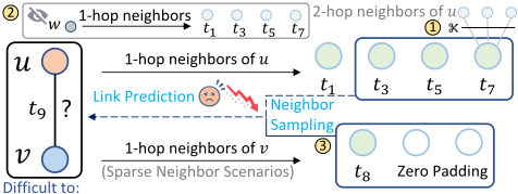
Figure 1: Illustration of three limitations of existing compression based neighbor sampling strategy for dynamic link prediction.
However, such compression based sampling methods suffers from the following three major limitations: (1) difficult to fully utilize the high order structural information. Since the size of neighborhoods grows exponentially with the increase of hops, multi-hop message passing will introduce prohibitive cost for large graphs. As a result, most existing methods only prune within one-hop historical neighbors, making them difficult to incorporate the high order structure information, as shown in the difficulty ① (upper right) of Figure 1; (2) difficult to fully utilize the temporal pattern information. As shown in the difficulty ② (upper left) of Figure 1, nodes w and u have never interacted, but they exhibit similar temporal interaction patterns at [t1, t3, t5, t7], which may indicate potential future interactions. This intuition is supported by previous studies showing that social network users who are consistently active in the same time period are more likely to become friends in the future [Cho et al., 2011]. However, such temporal patterns are largely ignored by existing methods. (3) difficult to learn the reliable representations for the nodes with sparse neighbors. Since dynamic graphs in real world are typically long tailed and intermittent, many nodes may have scarce or even no historical interactions with other nodes at some time points [Leskovec et al., 2005; Leskovec et al., 2010]. In this case, compression based sampling method often degenerates the input into short sequences or heavy padding, as shown in the difficulty ③ (lower right) of Figure 1. This leaves the model without sufficient context, making it difficult to learn reliable node representations.
To address these limitations, we rethink neighbor sampling from Compression to Context Construction. Specifically, instead of modifying the real neighbor sampling, we try to construct the interaction context with pseudo neighbor augmentation. The augmented pseudo neighbors provide auxiliary structural and temporal cues, and thus help to produce more stable temporal representations, especially for the nodes with scarce historical interaction. However, it is non-trivial to construct such pseudo neighbors due to the following challenges: (1) Limited informativeness. Weakly relevant pseudo neighbors may bring little useful context, leading to little gain or even misleading the model. (2) Efficiency bottleneck. Inefficient pseudo neighbor construction can be time-consuming, substantially increasing the computational cost. (3) Bias issue. Since pseudo and real neighbors differ in generation mechanisms , directly encoding them together may introduce bias, resulting in unreliable node representations.
To address these challenges, we propose a Pseudo Neighbor Augmentation Sampling Strategy based approach named PeNS for dynamic link prediction. Specifically, we first construct three complementary types of pseudo neighbors to inject high order structural (via structural bridge pseudo neighbors and shared hub pseudo neighbors) and temporal pattern (via temporal correlation pseudo neighbors) information into the interaction sequence context without introducing additional multi-hop message passing overhead. To efficiently construct pseudo neighbors, we further propose a Streaming Neighbor Memory Module that only requires a single chronological linear pass over the global edge stream to obtain the historical neighbor sequence at a given timestamp. Finally, we adopt a dual-stream fusion mechanism that encodes real and pseudo sequences separately, with cross attention for adaptive fusion to produce robust node representations. Our main contributions are summarized as follows.
- We present a novel perspective on neighbor sampling from Compression to Context Construction, thus providing richer interaction context for dynamic link prediction even when nodes have sparse interaction neighbors.
- We propose the Pseudo Neighbor Augmentation Sampling Strategy, which is plug-and-play and can be integrated into existing models. Based on this strategy, we further design an approach named PeNS to learn stable temporal representations for dynamic link prediction.
- Extensive experiments on multiple datasets demonstrate the effectiveness of our approach. Moreover, the consistent gains achieved when integrating our strategy into existing approaches further highlight its generalizability.
2 RelatedWork
DynamicGraphLearning. Dynamic graph learningmethods can be broadly categorized into discrete-time dynamic graph (DTDG) methods and continuous-time dynamic graph (CTDG) methods. DTDG methods [Seo et al., 2018; Hajiramezanali et al., 2019; Chen et al., 2022; Pareja et al., 2020; Sankar et al., 2018; Le and Ta, 2024; Yu et al., 2025] treat a dynamic graph as a sequence of static graph snapshots and then learn representations using static graph learning technique [Scarselli et al., 2008; Kipf and Welling, 2017; Veliˇckovi´c et al., 2018; Xu et al., 2019]. However, these methods rely on temporal discretization, which may discard event-level information. In contrast, CTDG methods [Poursafaei et al., 2022; Cong et al., 2023; Yu et al., 2023; Zou et al., 2024; Zhou et al., 2025] directly model on temporal event streams with continuous timestamps, preserving accurate interaction order and time intervals at the event level, thereby modeling dynamic evolution more faithfully.
Neighbor Sampling Strategy. Neighbor sampling strategies [Liu et al., 2021; Chen et al., 2018] aim to reduce the computational complexity by approximating the message passing on the full graph. Existing sampling methods can be categorized into three groups. Early works [Chen et al., 2017; Ying et al., 2018] adopt mini-batch recursive sampling, which first collect neighbors of nodes within a batch, expand layer by layer and then sample the full neighborhood at each layer. Another research line [Chen et al., 2019; Hamilton et al., 2017] focuses on node-wise sampling, which randomly selects at most k neighbors from the neighborhood of each node to approximate the node distribution of the full graph. Recent methods [Abu-El-Haija et al., 2023; Zeng et al., 2020] target at partitioned graphs and discard boundary nodes from other partitions while maintaining the connectivity among nodes within the batch.
3 Preliminaries
In this section, we present the definition of dynamic graphs and the formalization of dynamic link prediction.
Definition 1. Dynamic Graphs. A dynamic graph can be modeled as a time-ordered sequence of interaction events, denoted as G = {(u1, v1, t1), (u2, v2, t2), . . . , (uk, vk, tk)}, where 0 ≤ t1 ≤ t2 ≤ · · · ≤ tk represent the timestamps. Here, ui and vi denote the interaction nodes, indicating that nodes ui and vi interact at time ti. The node set is denoted by N . For each node u ∈ N , the node feature of u is represented as xu ∈ RdN . Moreover, each interaction event (u, v, t) has an edge feature xtu,v ∈ RdE , where dN and dE denote the dimensions of node and edge features, respectively.
Definition 2. Dynamic Link Prediction. Given two nodes u and v, a timestamp t, and the interaction history {(u′ , v′ , t′ ) | t′ < t} before t in a dynamic graph G, the goal of dynamic link prediction is to learn a mapping function f : (u, v, t) → ˆ ytu,v ∈ [0, 1], which estimates the interaction probability ˆ ytu,v and further predicts whether u and v will interact at time t.
4 Methodology
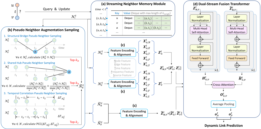
In this section, we illustrate the overall architecture of the proposed PeNS in Figure 2. Firstly, we query and update the Streaming Neighbor Memory Module (Sec 4.1) to obtain the real historical neighbor sequences. Then we augment the sequences to inject rich context via Pseudo Neighbors Augmentation Sampling (Sec 4.2). Next, we adopt Feature Encoding and Alignment (Sec 4.3) for the neighbor sequences to fuse multi-source features. Finally, a Dual-Stream Fusion Transformer (Sec 4.4) is employed to learn robust temporal representations for Dynamic Link Prediction (Sec 4.5).
4.1 Streaming Neighbor MemoryModule
In dynamic link prediction, a model typically needs to quickly retrieve the historical neighbor sequences of nodes u and v before time t when processing a sample (u, v, t), so as to construct the context for temporal encoding. To avoid repeatedly searching over the global edge set, we employ a Streaming Neighbor Memory Module to maintain node interaction histories at a given time, as shown in Figure 2(a). Specifically, for each node u ∈ N , we maintain a deque Du with a maximum capacity of kneigh, where each element stores the interaction information δ = (v, t), including the target node v and the interaction time t. When processing the event (u, v, t), we first query the historical neighbor sequences as follows:
where Read(·) returns a sequence with length at most kneigh. We then update the memory as:
If the sequence length exceeds kneigh, the oldest element is removed to keep the fixed capacity. This ensures that each edge triggers only a constant number of enqueue and dequeue operations, efficiently supporting the real neighbor retrieval and subsequent pseudo neighbor augmentation.
4.2 Pseudo Neighbor Augmentation Sampling
In this part, we design three complementary pseudo neighbor sampling strategies. These strategies can inject high order structural and temporal pattern information into interaction context without introducing additional multi-hop message passing overhead. To control the number of pseudo neighbors in each category, we adopt a Top-k scheme to keep the augmentation budget bounded. Given the real neighbor sequences N tu and N t v for a target sample (u, v, t), we sample pseudo neighbors as follows.
Structural Bridge PseudoNeighbor Sampling. As shown in the upper part of Figure 2(b), structural bridge pseudo neighbors inject cross-neighborhood bridging roles into the sequence. Specifically, for each node a ∈ N t v , we query its historical neighbors N t a from the previous presented Streaming Neighbor Memory Module, and compute the structural bridge score of node a as:
We then select the Top-kb nodes with the highest scores to form the structural bridge pseudo neighbor sequence ˜N tu,bridge . In particular, for attributed graphs, the interaction time and edge feature of a pseudo edge are computed as:
where tu,v denotes the interaction time between nodes u and v, and xtu,v denotes the edge feature of interaction (u, v, t).
The ˜N t v,bridge and its corresponding pseudo edge interaction times and edge features are computed analogously.
SharedHubPseudoNeighbor Sampling. As shown in the middle part of Figure 2(b), shared hub pseudo neighbors select highly connected nodes that are commonly associated with both endpoints, serving as stable contextual anchors especially for sparse interaction nodes. Specifically, for each node a ∈ N, we compute its overlap sizes ru(a) and rv(a) with the neighborhoods of both endpoints u and v as:
and obtain the shared hub score via max normalization as:
where ϵ is a small positive constant to avoid division by zero. For computational simplicity, we restrict a ∈ N tu ∪ N t v .
We then select the Top-kh nodes to form the shared hub pseudo neighbor sequence ˜N tu,v,hub , and append it to both the pseudo neighbor sequences of nodes u and v. In particular, for attributed graphs, the pseudo edge interaction time and edge feature are computed as:
Temporal Correlation Pseudo Neighbor Sampling. As shown in the lower part of Figure 2(b), temporal correlation pseudo neighbors exploit temporal correlations in interaction sequences, enabling the model to observe potentially related interaction partners and thus better capture temporal interaction patterns. Specifically, we denote the historical interaction timestamp sequence of node u at time t as TN tu = (tu,1, tu,2, . . . , tu,m), and construct its adjacentinterval sequence ∆TN tu = (tu,2 - tu,1, . . . , tu,m - tu,m-1), where m ≤ kneigh. For each node a ∈ N, we compute its temporal correlation score with respect to node u as:
where PCC(·) computes the Pearson Correlation Coefficient between two sequences. For computational simplicity, we restrict a ∈ N tu ∪N t v as shared hub pseudo neighbor sampling.
We then select the Top-kc nodes with the highest scores to form the temporal correlation pseudo neighbor sequence ˜N tu,corr . In particular, for attributed graphs, the pseudo edge interaction time and edge feature are computed as:
The ˜N t v,corr and its corresponding pseudo edge interaction times and edge features are computed analogously.
Finally, we concatenate the three types of pseudo neighbors to obtain the final pseudo neighbor sequences as:
4.3 Feature Encoding and Alignment
To uniformly characterize the information carried by real and pseudo neighbors, we construct a joint representation that includes node, edge, time, frequency, and source information, as shown in Figure 2(c).
For each a ∈ N tu , we define the relative time ∆ta = t-tu,a and introduce a source label sa ∈ {real,bridge,hub,corr}. The node feature xa ∈ RdN and the edge feature xtu,a u,a ∈ RdE are obtained from the dynamic graph G. Following [Cong et al., 2023], we derive the time representation by mapping ∆ta into a continuous vector via cosine functions as:
where wi is a fixed node-specific feature and dT denotes the dimension of time encoding.
The frequency feature explicitly models the intensity of repeated interactions. Given the four neighbor sequences, the frequency feature of node a is computed as:
where N tu (a) denotes the number of occurrences of node a in the sequence N tu .
The source feature xta,S indicates whether the neighbor comes from the real sequence or one of three pseudo neighbor types, obtained by one-hot encoding the source label sa.
Finally, we feed these features into separate linear layers to align them to dimension d, and then concatenate them to obtain the neighbor sequence representations Ztu = Xtu,N ||Xtu,E ||Xtu,T ||Xtu,F ||Xtu,S ∈ Rkneigh×5d . Stacking the representations of both endpoints yields the interaction representation Ztu,v = [Ztu ;Ztv ] ∈ R2kneigh×5d . Similarly, we obtain ˜Ztu,v = [ ˜Ztu ; ˜Ztv ] ∈ R2kpseudo×5d , where kpseudo = kb + kh + kc denotes the total number of pseudo neighbors. Positions with insufficient length are padded with zeros for dimensional alignment.
4.4 Dual-StreamFusion Transformer
In our framework, real neighbors provide observed signal while pseudo neighbors act as prior supplements. They differ in their generation mechanisms and noise characteristics. Directly mix and feed them into a single encoder may introduce bias, which can mislead temporal representation learning. Hence, we adopt a Dual-Stream Fusion Transformer as shown in Figure 2(d), where two structurally identical but parameter-independent Transformer [Vaswani et al., 2017] encoders are used to learn the representationsHtu,v and ˜Htu,v of real stream and pseudo stream respectively as follows:
Then, to allow the real interaction to adaptively absorb the structural and temporal priors injected by pseudo neighbors, we perform cross-attention fusion by using the real stream as query and the pseudo stream as key and value, yielding the fused interaction representation matrix as:
The final temporal representations otu and otv of nodes u and v at time t are obtained by averaging their corresponding rows in Otu,v and applying a linear projection as:
whereWout ∈ R5d×dout and bout ∈ Rdout are learnable parameters, and dout denotes the output dimension.
4.5 Dynamic Link Prediction
After obtaining the temporal representations otu and otv and concatenating them, we predict the interaction probability via a multi-layer perceptron (MLP) [Rumelhart et al., 1986] as:
We adopt the binary cross-entropy loss for supervision as:
where E + and E - denote the sets of positive and negative samples, respectively, and N is the total number of samples.
5 Experiments
In this section, extensive experiments are conducted. We report results for various baselines and further demonstrate the generalizability of our sampling strategy by equipping it into existing methods. We then provide an in-depth analysis on the effect of key hyperparameters and components.
5.1 Experimental Settings
Datasets. We evaluate PeNS on 9 real-world dynamic graph datasets (i.e., Wikipedia, Reddit, MOOC, LastFM, Enron, UCI, BITotc, BITalpha, and DBLP) from [Poursafaei et al., 2022; Xu et al., 2023].
Baselines. We compare PeNS against 11 widely used dynamic graph methods, including four memory-based methods (JODIE [Kumar et al., 2019], DyRep [Trivedi et al., 2019], TGN [Rossi et al., 2020], and PANet [Zhou et al., 2025]), a graph convolution-based method (TGAT [Xu et al., 2020]), a random-walk-based method (CAWN [Wang et al., 2021b]), a statistical method (EdgeBank [Poursafaei et al., 2022]), two MLP-based methods (GraphMixer [Cong et al., 2023] and RepeatMixer [Zou et al., 2024]), and two sequence-based methods (TCL [Wang et al., 2021a] and DyGFormer [Yu et al., 2023]).
Evaluation Tasks and Metrics. We consider two settings: (1) transductive dynamic link prediction, which predicts links between nodes observed during training period, and (2) inductive dynamic link prediction, which predicts links involving previously unseen nodes. Negative samples are randomly selected with a 1:1 ratio to positive samples. We report Average Precision (AP) and Area Under the Receiver Operating Characteristic Curve (AUC-ROC) as the main metrics.
Implementation Details. We use the same hyperparameter settings as those in DyGLib [Yu et al., 2023] for fair comparison. Our code is available at https://github.com/CsuYuzhigang/PeNS.
5.2 Performance Comparison
Overall Performance. We report the comparison results for dynamic link prediction in Table 1. Based on the results, we make the following key observations:
(i) Under the transductive setting, PeNS achieves almost consistent SOTA performance across datasets. In terms of AP, PeNS outperforms the strongest baseline by 5.71% on LastFM, 3.31% on UCI and 8.53% on DBLP. Moreover, on datasets that are close to saturation (e.g., Wikipedia and Reddit), PeNS still pushes performance to around 99.9% on top of very strong baselines, demonstrating its effectiveness.
(ii) Under the more challenging inductive setting, the advantages of PeNS become even more pronounced. In terms of AP, PeNS improves upon the strongest baseline by at least 10% on datasets such as BITotc (97.86%), BITalpha (97.29%) and DBLP (93.39%). This suggests that when many unseen nodes appear at test time, conventional methods rely more heavily on retrievable real historical interactions to form representations. In contrast, PeNS leverages the enriched context brought by augmentation to provide more stable signals when real neighbors are insufficient, thereby largely preventing the severe performance drop on nodes with sparse interactions. Although PeNS does not achieve the best result on MOOC, it delivers more stable performance and a higher lower bound on most datasets.
Overall, these results support our core motivation: the key bottleneck in dynamic graph learning is not only the need to compress overly many neighbors, but also the lack of sufficient context. This bottleneck becomes more pronounced in inductive settings or sparse neighbor scenarios. PeNS effectively complements structural and temporal information through pseudo neighbor augmentation and dual-stream fusion, leading to significant and stable performance gains.
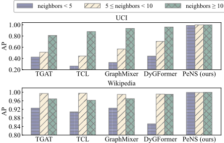
Performance under Varying Neighbor Availability. We conduct an evaluation stratified by historical interaction neighbor availability to compare PeNS with existing baselines. The results are shown in Figure 3.
Specifically, we partition the test samples into three groups according to the number of historical neighbors of the anchor node at the target time, and then report the AP of methods across different groups to examine performance differences under varying neighbor availability. The results show that when sufficient historical neighbors are available (neighbors ≥ 10), all four baselines achieve relatively strong performance on both datasets. In contrast, when historical neighbors are extremely sparse (neighbors < 5), the performance of these baselines drops significantly, indicating that the models rely heavily on limited historical interaction information and struggle to construct stable temporal representations in sparse conditions. In contrast, by augmenting with pseudo neighbors, PeNS achieves performance in sparse scenarios that is comparable to that in dense scenarios, while consistently outperforming baselines across all scenarios, indicating the effectiveness and generalizability of our approach.
| Settings | Metrics | Datasets | JODIE | DyRep | TGAT | TGN | CAWN | EdgeBank | TCL | GraphMixer | DyGFormer | PANet | ||
|---|---|---|---|---|---|---|---|---|---|---|---|---|---|---|
| AP | Wikipedia Reddit MOOC LastFM Enron UCI BITotc BITalpha DBLP Wikipedia Reddit MOOC LastFM Enron UCI | 96.51 ± 0.19 98.32 ± 0.06 81.34 ± 1.64 70.72 ± 2.25 84.04 ± 3.23 90.00 ± 1.40 89.64 ± 0.25 88.65 ± 0.25 80.70 ± 0.38 96.34 ± 0.11 98.29 ± 0.04 84.39 ± 1.31 70.78 ± 1.12 87.05 ± 2.69 | 94.72 ± 0.21 98.20 ± 0.05 80.93 ± 1.15 68.84 ± 5.73 78.96 ± 3.53 65.85 ± 4.14 81.91 ± 0.69 78.12 ± 1.43 78.51 ± 0.86 94.39 ± 0.16 98.16 ± 0.04 84.09 ± 1.20 68.08 ± 5.41 82.15 ± 2.91 70.85 ± 3.01 83.30 ± 0.90 78.49 ± 0.90 | 96.81 ± 0.09 98.52 ± 0.01 85.42 ± 0.11 73.11 ± 0.14 71.42 ± 1.27 79.99 ± 1.00 91.01 ± 0.97 85.81 ± 2.00 75.02 ± 1.80 96.52 ± 0.10 98.46 ± 0.01 86.73 ± 0.14 71.29 ± 0.20 69.13 ± 1.69 79.09 ± 1.22 91.11 ± 0.93 84.43 ± 2.28 77.94 ± 1.34 | 98.33 ± 0.08 98.58 ± 0.05 90.26 ± 0.79 74.41 ± 3.38 87.56 ± 0.67 92.86 ± 0.59 92.36 ± 0.69 88.51 ± 1.69 83.76 ± 1.32 98.25 ± 0.09 98.53 ± 0.07 92.07 ± 0.56 75.91 ± 2.83 89.32 ± 0.66 92.65 ± 0.69 92.26 ± 0.78 87.88 ± 1.91 84.62 ± 1.11 | 98.76 ± 0.03 99.10 ± 0.01 80.56 ± 0.23 86.99 ± 0.06 89.56 ± 0.07 95.06 ± 0.16 94.05 ± 0.13 91.00 ± 0.21 89.25 ± 0.08 98.54 ± 0.04 99.01 ± 0.01 80.81 ± 0.21 85.92 ± 0.10 90.41 ± 0.10 93.70 ± 0.21 94.10 ± 0.16 91.42 ± 0.16 87.83 ± 0.10 | 90.37 ± 0.00 94.86 ± 0.00 57.97 ± 0.00 79.29 ± 0.00 83.53 ± 0.00 76.20 ± 0.00 50.00 ± 0.00 50.00 ± 0.00 56.27 ± 0.00 90.78 ± 0.00 95.37 ± 0.00 60.86 ± 0.00 83.77 ± 0.00 87.05 ± 0.00 77.30 ± 0.00 49.83 ± 0.00 49.80 ± 0.00 56.28 ± 0.00 | 96.16 ± 0.21 97.54 ± 0.01 82.23 ± 0.33 65.31 ± 1.56 78.25 ± 2.78 86.12 ± 1.40 94.01 ± 0.17 91.95 ± 0.24 76.89 ± 0.49 95.45 ± 0.20 97.43 ± 0.01 83.03 ± 0.28 62.32 ± 1.70 74.24 ± 3.02 85.15 ± 0.90 94.22 ± 0.17 92.10 ± 0.10 | 96.95 ± 0.03 97.43 ± 0.02 83.46 ± 0.16 74.60 ± 1.88 81.80 ± 0.34 93.01 ± 0.45 93.99 ± 0.19 91.56 ± 0.12 73.63 ± 0.77 96.64 ± 0.03 97.35 ± 0.02 84.81 ± 0.12 72.40 ± 2.24 84.25 ± 0.19 91.41 ± 0.59 94.25 ± 0.16 91.57 ± 0.15 | 99.02 ± 0.02 99.21 ± 0.01 87.37 ± 0.51 93.09 ± 0.05 92.34 ± 0.20 95.86 ± 0.05 94.26 ± 0.17 90.86 ± 0.27 89.22 ± 0.09 98.91 ± 0.03 99.14 ± 0.01 87.78 ± 0.48 93.15 ± 0.02 93.09 ± 0.29 94.59 ± 0.06 94.12 ± 0.17 90.20 ± 0.62 87.81 ± 0.12 | RepeatMixer 99.11 ± 0.02 99.18 ± 0.01 92.31 ± 0.20 93.99 ± 0.08 92.27 ± 0.05 96.54 ± 0.09 95.00 ± 0.04 91.71 ± 0.31 86.09 ± 0.10 99.00 ± 0.02 99.09 ± 0.02 93.28 ± 0.16 93.97 ± 0.02 93.04 ± 0.17 95.55 ± 0.13 94.90 ± 0.08 91.47 ± 0.48 84.39 ± 0.13 | 98.67 ± 0.03 98.85 ± 0.02 90.77 ± 1.86 90.31 ± 0.51 91.59 ± 0.19 95.35 ± 0.23 93.40 ± 0.57 89.58 ± 1.11 83.44 ± 1.58 98.53 ± 0.03 98.80 ± 0.02 92.34 ± 1.55 89.74 ± 0.51 93.04 ± 0.15 94.36 ± 0.37 93.29 ± 0.62 88.29 ± 1.63 83.09 ± 1.75 | PeNS (ours) 99.96 ± 0.01 99.91 ± 0.01 93.12 ± 0.08 99.36 ± 0.01 94.93 ± 0.23 99.74 ± 0.10 99.40 ± 0.08 99.33 ± 0.18 96.86 ± 0.66 99.96 ± 0.01 99.94 ± 0.01 94.16 ± 0.05 99.46 ± 0.02 96.17 ± 0.25 99.76 ± 0.10 99.46 ± 0.09 99.29 ± 0.16 96.50 ± 0.62 | |
| TRA | ||||||||||||||
| AUC | ||||||||||||||
| 90.91 ± 0.88 | ||||||||||||||
| BITotc | 91.06 ± 0.17 | |||||||||||||
| BITalpha | 89.62 ± 0.13 | |||||||||||||
| DBLP | 82.53 ± 0.26 | 80.37 ± 0.65 | 79.59 ± 0.25 | 76.42 ± 0.63 | ||||||||||
| AP | Wikipedia | 94.68 ± 0.17 | 92.00 ± 0.32 | 96.17 ± 0.07 | 97.68 ± 0.16 | 98.24 ± 0.02 | - | 95.90 ± 0.27 | 96.42 ± 0.02 | 98.60 ± 0.03 | 98.69 ± 0.02 | 98.18 ± 0.02 | 99.88 ± 0.04 | |
| 96.64 ± 0.31 | 95.87 ± 0.08 | 97.08 ± 0.05 | 97.40 ± 0.10 | 98.61 ± 0.01 | - | 94.19 ± 0.09 | 95.14 ± 0.07 | 98.82 ± 0.01 | 98.80 ± 0.02 | 98.51 ± 0.04 | 99.81 ± 0.02 | |||
| MOOC | 80.61 ± 1.26 | 80.37 ± 0.95 | 85.07 ± 0.17 | 89.67 ± 0.94 | 81.65 ± 0.14 | - | 80.51 ± 0.43 | 82.42 ± 0.25 | 86.97 ± 0.53 | 92.34 ± 0.20 | 89.98 ± 2.11 | 90.92 ± 0.07 | ||
| LastFM | 82.90 ± 1.08 | 80.57 ± 4.40 | 78.23 ± 0.20 | 79.05 ± 2.92 | 89.42 ± 0.07 | - | 70.63 ± 3.43 | 79.67 ± 3.73 | 94.26 ± 0.08 | 94.97 ± 0.14 | 93.28 ± 0.16 88.38 ± 0.37 | 99.00 ± 0.02 | ||
| Enron | 80.68 ± 1.47 | 73.59 ± 4.10 | 66.84 ± 1.26 | 78.63 ± 2.61 88.62 ± 0.78 | 86.17 ± 0.21 | - | 74.37 ± 3.07 | 75.96 ± 0.86 | 89.78 ± 0.55 | 88.26 ± 0.14 | 92.06 ± 0.41 | 92.53 ± 0.45 | ||
| UCI | 79.33 ± 2.86 | 58.16 ± 2.70 | 79.56 ± 1.19 | 92.50 ± 0.20 | - | 83.70 ± 1.45 | 91.17 ± 0.17 | 94.54 ± 0.07 | 95.01 ± 0.08 86.07 ± 0.21 | 83.78 ± 0.41 | 99.16 ± 0.21 97.86 ± 0.08 | |||
| BITotc | 72.09 ± 0.27 | 64.83 ± 0.97 | 81.56 ± 0.61 | 82.62 ± 1.24 | 84.18 ± 0.16 | - | 83.52 ± 0.38 | 82.97 ± 0.24 | 85.11 ± 0.33 | |||||
| BITalpha | 70.93 ± 0.42 | 63.82 ± 2.08 | 72.51 ± 1.18 | 74.63 ± 0.55 | 76.03 ± 0.47 | - | 77.35 ± 0.67 | 76.87 ± 0.30 | 77.13 ± 0.29 | 78.79 ± 0.14 | 76.85 ± 0.24 | 97.29 ± 0.43 | ||
| DBLP | 64.37 ± 0.77 | 63.24 ± 1.46 | 57.45 ± 2.05 | 69.62 ± 1.77 | 77.06 ± 0.11 | - | 59.08 ± 0.21 | 55.73 ± 0.37 | 77.18 ± 0.04 | 73.15 ± 0.05 | 74.77 ± 0.84 | 93.39 ± 2.93 | ||
| IND | AUC | Wikipedia | 94.20 ± 0.11 | 91.05 ± 0.41 | 95.85 ± 0.08 | 97.57 ± 0.17 | 98.03 ± 0.03 | - | 95.22 ± 0.25 | 96.05 ± 0.04 | 98.51 ± 0.04 | 98.59 ± 0.01 | 98.05 ± 0.04 | 99.90 ± 0.03 |
| 96.67 ± 0.20 | 95.92 ± 0.09 | 96.98 ± 0.07 | 97.29 ± 0.12 | 98.42 ± 0.02 | - | 93.87 ± 0.14 | 94.89 ± 0.10 | 98.69 ± 0.02 | 98.62 ± 0.02 | 98.40 ± 0.03 | 99.84 ± 0.02 | |||
| MOOC | 83.61 ± 1.01 | 83.42 ± 0.68 | 86.41 ± 0.13 | 91.49 ± 0.64 | 82.12 ± 0.15 | - | 81.42 ± 0.38 | 83.89 ± 0.19 | 87.61 ± 0.51 | 93.38 ± 0.16 | 91.50 ± 1.68 | 92.07 ± 0.03 | ||
| LastFM | 82.10 ± 1.15 | 80.12 ± 3.98 | 76.58 ± 0.25 | 80.12 ± 2.29 | 87.82 ± 0.12 | - | 68.40 ± 3.12 | 77.55 ± 4.55 | 94.14 ± 0.04 | 94.89 ± 0.03 | 92.92 ± 0.12 | 99.16 ± 0.02 | ||
| Enron | 82.28 ± 1.70 | 75.74 ± 3.20 | 64.38 ± 1.19 | 79.55 ± 2.57 | 86.98 ± 0.16 | - | 70.77 ± 3.40 | 76.89 ± 0.80 | 90.72 ± 0.61 | 88.62 ± 0.20 | 89.23 ± 0.13 | 93.93 ± 0.34 | ||
| UCI | 78.58 ± 2.26 | 60.02 ± 2.37 | 77.76 ± 1.23 | 87.36 ± 1.03 | 90.08 ± 0.28 | - | 81.33 ± 1.15 | 89.32 ± 0.21 | 92.57 ± 0.11 | 93.47 ± 0.10 | 89.84 ± 0.66 | 99.14 ± 0.23 | ||
| BITotc | 70.13 ± 0.50 | 63.67 ± 0.69 | 80.34 ± 0.22 | 81.03 ± 0.75 | 81.23 ± 0.11 | - | 81.41 ± 0.20 | 81.09 ± 0.16 | 82.26 ± 0.48 | 83.38 ± 0.26 | 82.43 ± 0.28 | 97.45 ± 0.10 | ||
| BITalpha | 70.27 ± 0.38 | 63.30 ± 0.99 | 71.06 ± 1.31 | 73.15 ± 0.70 | 73.41 ± 0.52 | - | 74.77 ± 0.29 | 74.20 ± 0.37 | 73.99 ± 0.48 | 75.59 ± 0.35 | 75.00 ± 0.34 | 96.94 ± 0.45 | ||
| DBLP | 63.82 ± 0.98 | 63.31 ± 1.51 | 59.00 ± 2.00 | 70.37 ± 1.49 | 73.70 ± 0.12 | - | 59.44 ± 0.18 | 55.93 ± 0.54 | 73.95 ± 0.06 | 69.45 ± 0.13 | 72.69 ± 1.16 | 93.14 ± 2.65 |
5.3 Effects of Pseudo Neighbor Augmentation Sampling Strategy
To investigate the impact of our Pseudo Neighbor Augmentation Sampling Strategy, we conduct two experiments from the perspectives of generalizability and effectiveness.
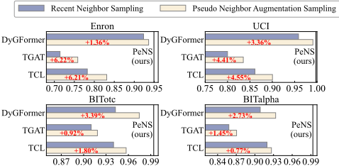
Generalizability of Pseudo Neighbor Augmentation Sampling Strategy. We integrate the proposed sampling strategy into different baselines (DyGFormer, TGAT, and TCL), and report AP results on transductive dynamic link prediction in Figure 4. The results show consistent improvements across four datasets, indicating that neighbor augmentation can provide effective contextual signals without modifying the core modeling components of the baselines, thus yielding broad gains across models and datasets. Moreover, the improvement magnitude is closely related to both the representational capacity of the backbone model and the interaction sparsity of the dataset. The gains are more evident when the original method is more sensitive to context information or more likely to suffer from insufficient historical neighbors.
Comparison with Different Variants. Table 2 compares three variants: using our designed pseudo neighbors (Ours), using random pseudo neighbors (Random), and replacing pseudo neighbors with more real neighbors (Real). The results demonstrate that our carefully designed pseudo neighbors provide informative context and improve temporal representation learning. In contrast, randomly introduced pseudo neighbors tend to inject substantial noise and fail to offer useful complementary signals. Thanks to the dual-stream fusion mechanism, the model adaptively balances real and pseudo neighbors, suppressing irrelevant information and maintaining stable performance. While replacing with more real neighbors avoids random noise, it is still insufficient to compensate for the missing context in sparse neighbor scenarios and mitigate the loss of structural and temporal information.
| Transductive | Inductive | |||||
|---|---|---|---|---|---|---|
| Datasets | Ours | Random | Real | Ours | Random | Real |
| Wikipedia | 99.96 ± 0.01 | 98.11 ± 0.01 | 98.76 ± 0.02 | 99.88 ± 0.04 | 97.59 ± 0.03 | 98.35 ± 0.03 |
| 99.91 ± 0.01 | 98.26 ± 0.02 | 98.83 ± 0.01 | 99.81 ± 0.02 | 98.04 ± 0.04 | 98.55 ± 0.03 | |
| MOOC | 93.12 ± 0.08 | 87.48 ± 0.27 | 89.26 ± 0.06 | 90.92 ± 0.07 | 83.81 ± 0.34 | 86.08 ± 0.11 |
| LastFM | 99.36 ± 0.01 | 90.95 ± 0.05 | 92.51 ± 0.04 | 99.00 ± 0.02 | 90.28 ± 0.08 | 92.02 ± 0.06 |
| Enron | 94.93 ± 0.23 | 90.88 ± 0.23 | 92.11 ± 0.16 | 92.53 ± 0.45 | 84.16 ± 0.59 | 87.74 ± 0.53 |
| UCI | 99.74 ± 0.10 | 94.07 ± 0.24 | 95.86 ± 0.17 | 99.16 ± 0.21 | 92.64 ± 0.19 | 94.43 ± 0.19 |
| BITotc | 99.40 ± 0.08 | 93.84 ± 0.08 | 94.02 ± 0.15 | 97.86 ± 0.08 | 91.61 ± 0.11 | 92.53 ± 0.43 |
| BITalpha | 99.33 ± 0.18 | 86.50 ± 0.21 | 88.26 ± 0.25 | 97.29 ± 0.43 | 85.43 ± 0.12 | 87.40 ± 0.52 |
| DBLP | 96.86 ± 0.66 | 85.59 ± 0.17 | 87.01 ± 0.05 | 93.39 ± 2.93 | 75.53 ± 0.12 | 76.58 ± 0.04 |
5.4 Effects of Different Hyperparameters
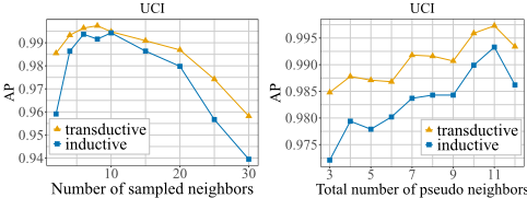
More specifically, we examine the effects of key hyperparameters on PeNS. Figure 5 reports the results on UCI.
Number of Sampled Neighbors. The left of Figure 5 shows that using few sampled neighbors yields insufficient context and limits the performance. As the number increases, the performance improves rapidly and then reaches its peak. However, further increasing this number leads to a gradual drop in AP, with a more clear degradation under the inductive setting. This suggests that overly long historical neighbor sequences introduce more outdated or weakly related interactions, interfering with temporal modeling, and the effect is more pronounced under inductive settings.
Total Number of Pseudo Neighbors. The right of Figure 5 shows that AP increases as the total number of pseudo neighbors grows, and the gain later plateaus or slightly declines. It indicates that a reasonable amount of pseudo neighbors can continuously provide effective context and improve representation quality, while too many pseudo neighbors increase computational cost and may introduce additional noise.
5.5 Ablation Study
To evaluate the effectiveness of individual components in PeNS, we conduct an ablation study with the following variants: w/o PN removes all pseudo neighbors; w/o SBN, w/o SHN, and w/o TCN remove structural bridge neighbors, shared hub neighbors, and temporal correlation neighbors, respectively; w/o FE removes frequency encoding; and w/o SE removes source encoding.
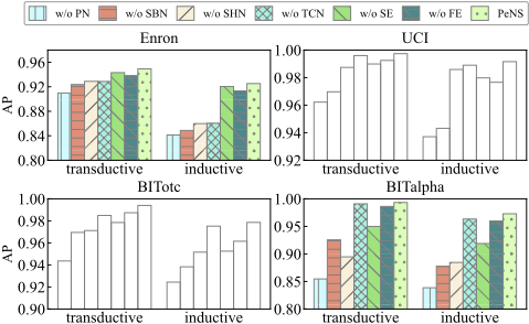
As shown in Figure 6, all variants perform worse than the full PeNS under both transductive and inductive settings, indicating that all these components work together and achieve the best performance when fully enabled. A closer look shows that removing pseudo neighbors (w/o PN) leads to the most pronounced drop (e.g., 5.07% in BITotc and 13.96% in BITalpha under transductive settings), suggesting that pseudo neighbor augmentation is the primary driver of the overall gains. Meanwhile, removing source encoding (w/o SE) also noticeably degrades performance (e.g., 4.37% drop in BITalpha under transductive settings), implying that explicitly distinguishing real neighbors from different types of pseudo neighbors helps the model utilize the augmented context in a stable and effective manner. Among the three kinds of pseudo neighbors, removing structural bridge neighbors (w/o SBN) or shared hub neighbors (w/o SHN) typically causes larger performance losses, highlighting the dominant role of high order structural information. Removing temporal correlation neighbors (w/o TCN) also yields consistent degradation, indicating that the injected temporal pattern signals complement structural information and remain indispensable. Finally, the results of w/o FE verify that modeling repeated interaction intensity provides additional useful signals for prediction.
6 Conclusion
In this paper, we rethink neighbor sampling from compression to context construction and propose PeNS. Specifically, we design a Pseudo Neighbor Augmentation Sampling Strategy that constructs three complementary types of pseudo neighbors. It can inject high order structural and temporal pattern information into the interaction context without introducing additional multi-hop message passing overhead, and generalize well to sparse neighbor scenarios. A Streaming Neighbor Memory Module is developed to construct pseudo neighbors efficiently. In addition, we adopt a dual-stream fusion mechanism to enable more stable temporal representations for dynamic link prediction. Extensive experiments demonstrate the effectiveness and generalizability of PeNS.
Acknowledgments
This research was funded by the National Natural Science Foundation of China (No.62572489 and No.72571284), Hunan Provincial Fund for Distinguished Young Scholars (No.2025JJ20073), Science and Technology Innovation Program of Hunan Province (No.2023RC3009) and Innovation Research Foundation of National University of Defense Technology (No.JS24-05).
@inproceedings{ijcai2026p585,
  title     = {From Compression to Construction: Pseudo Neighbor Augmentation Sampling for Dynamic Link Prediction},
  author    = {Yu, Zhigang and Yan, Hao and Fan, Changjun and Wang, Senzhang},
  booktitle = {Proceedings of the Thirty-Fifth International Joint Conference on
               Artificial Intelligence, {IJCAI-26}},
  publisher = {International Joint Conferences on Artificial Intelligence Organization},
  editor    = {Diego Calvanese},
  pages     = {5254--5262},
  year      = {2026},
  month     = {8},
  note      = {Main Track},
  doi       = {10.24963/ijcai.2026/585},
  url       = {https://doi.org/10.24963/ijcai.2026/585},
}
TY - CPAPER TI - From Compression to Construction: Pseudo Neighbor Augmentation Sampling for Dynamic Link Prediction AU - Yu, Zhigang AU - Yan, Hao AU - Fan, Changjun AU - Wang, Senzhang T2 - Proceedings of the Thirty-Fifth International Joint Conference on Artificial Intelligence, IJCAI-26 PB - International Joint Conferences on Artificial Intelligence Organization PY - 2026 SP - 5254 EP - 5262 DO - 10.24963/ijcai.2026/585 UR - https://doi.org/10.24963/ijcai.2026/585 ER -Copied
Machine-readable versions of this paper, for tools and AI agents:





