Disentangling Coarse and Fine Latent Dynamics for Probabilistic Time Series Forecasting

Zhou, Changze; Cai, Ruichu; Nie, Shengbin; Fang, Juntao; Qiao, Jie; Li, Zijian

doi:10.24963/ijcai.2026/602

Disentangling Coarse and Fine Latent Dynamics for Probabilistic Time Series Forecasting

Changze Zhou, Ruichu Cai, Shengbin Nie, Juntao Fang, Jie Qiao, Zijian Li

Download BibTeX Cite

Proceedings of the Thirty-Fifth International Joint Conference on Artificial Intelligence. Main Track. Pages 5404-5412.

https://doi.org/10.24963/ijcai.2026/602

Keywords

Machine Learning: Time series and data streams

Abstract

Probabilistic time series forecasting seeks to quantify the uncertainty of future observations. While recent works introduce latent variables to alleviate the spurious dependencies caused by hidden confounders, thereby reducing overly wide confidence intervals, simply incorporating latent factors is not sufficient. When the underlying latent dynamics evolve at multiple temporal scales, existing methods may entangle temporally coarse and fine latent dynamics, which introduces spurious latent transitions and in turn amplifies predictive uncertainty. Therefore, disentangling temporally coarse and fine latent dynamics is essential for achieving sharper and more reliable probabilistic forecasting results. Building on this insight, we propose COFE (COarse And FinE latent dynamics disentanglement), a variational autoencoder–based framework that models the temporal distribution by disentangling and modeling the rapidly changing and slowly varying latent dynamics simultaneously. In particular, the proposed COFE harnesses the independence of estimated noises between adjacent latent states as well as a sparsity constraint on estimated noise to disentangle latent dynamics across different scales effectively. More specifically, we show that the multi-scale latent dynamics are disentangled with rigorous theoretical guarantees. Extensive experiments on 15 benchmark datasets, compared against 12 state-of-the-art baselines, demonstrate that COFE achieves superior uncertainty quantification, validating its effectiveness in a wide range of real-world scenarios. Code is available at https://github.com/polars8948/COFE

[Bacanin et al., 2023] Nebojsa Bacanin, Luka Jovanovic, Miodrag Zivkovic, Venkatachalam Kandasamy, Milos An- tonijevic, Muhammet Deveci, and Ivana Strumberger. Multivariate energy forecasting via metaheuristic tuned long-short term memory and gated recurrent unit neural networks. Information Sciences, 642:119122, 2023.
[Bergsma et al., 2022] Shane Bergsma, Tim Zeyl, Javad Rahimipour Anaraki, and Lei Guo. C2far: Coarse-to-fine autoregressive networks for precise probabilistic forecast- ing. Advances in Neural Information Processing Systems, 35:21900-21915, 2022.
[Daunhawer et al., 2023] Imant Daunhawer, Alice Bizeul, Emanuele Palumbo, Alexander Marx, and Julia E Vogt. Identifiability results for multimodal contrastive learning. arXiv preprint arXiv:2303.09166, 2023.
[Hyvarinen and Morioka, 2016] Aapo Hyvarinen and Hi- roshi Morioka. Unsupervised feature extraction by time- contrastive learning and nonlinear ica. Advances in neural information processing systems, 29, 2016.
[Hyvärinen and Pajunen, 1999] Aapo Hyvärinen and Petteri Pajunen. Nonlinear independent component analysis: Existence and uniqueness results. Neural networks, 12(3):429-439, 1999.
[Jhin et al., 2024] Sheo Yon Jhin, Seojin Kim, and Noseong Park. Addressing prediction delays in time series forecast- ing: A continuous gru approach with derivative regular- ization. In Proceedings of the 30th ACM SIGKDD Con- ference on Knowledge Discovery and Data Mining, KDD '24, page 1234-1245, New York, NY, USA, 2024. Associ- ation for Computing Machinery.
[Khemakhem et al., 2020] Ilyes Khemakhem, Diederik Kingma, Ricardo Monti, and Aapo Hyvarinen. Variational autoencoders and nonlinear ica: A unifying framework. In International conference on artificial intelligence and statistics, pages 2207-2217. PMLR, 2020.
[Kollovieh et al., 2023] Marcel Kollovieh, Abdul Fatir Ansari, Michael Bohlke-Schneider, Jasper Zschiegner, Hao Wang, and Yuyang Bernie Wang. Predict, refine, synthesize: Self-guiding diffusion models for probabilistic time series forecasting. Advances in Neural Information Processing Systems, 36:28341-28364, 2023.
[Kollovieh et al., 2024] Marcel Kollovieh, Marten Lienen, David Lüdke, Leo Schwinn, and Stephan Günnemann. Flow matching with gaussian process priors for prob- abilistic time series forecasting. arXiv preprint arXiv:2410.03024, 2024.
[Kong et al., 2022] Lingjing Kong, Shaoan Xie, Weiran Yao, Yujia Zheng, Guangyi Chen, Petar Stojanov, Victor Akin- wande, and Kun Zhang. Partial disentanglement for do- main adaptation. In International conference on machine learning, pages 11455-11472. PMLR, 2022.
[Lachapelle et al., 2023] Sébastien Lachapelle, Tristan Deleu, Divyat Mahajan, Ioannis Mitliagkas, Yoshua Bengio, Simon Lacoste-Julien, and Quentin Bertrand. Synergies between disentanglement and sparsity: Gen- eralization and identifiability in multi-task learning. In International Conference on Machine Learning, pages 18171-18206. PMLR, 2023.
[Lai et al., 2018] Guokun Lai, Wei-Cheng Chang, Yiming Yang, and Hanxiao Liu. Modeling long-and short-term temporal patterns with deep neural networks. In The 41st international ACM SIGIR conference on research & devel- opment in information retrieval, pages 95-104, 2018.
[Li et al., 2022] Yan Li, Xinjiang Lu, Yaqing Wang, and De- jing Dou. Generative time series forecasting with diffu- sion, denoise, and disentanglement. Advances in Neural Information Processing Systems, 35:23009-23022, 2022.
[Li et al., 2024a] Yuxin Li, Wenchao Chen, Xinyue Hu, Bo Chen, Mingyuan Zhou, et al. Transformer-modulated diffusion models for probabilistic multivariate time series forecasting. In The Twelfth International Conference on Learning Representations, 2024.
[Li et al., 2024b] Zijian Li, Yifan Shen, Kaitao Zheng, Ruichu Cai, Xiangchen Song, Mingming Gong, Zheng- mao Zhu, Guangyi Chen, and Kun Zhang. On the iden- tification of temporally causal representation with instan- taneous dependence. arXiv preprint arXiv:2405.15325, 2024.
[Li et al., 2025] Qi Li, Zhenyu Zhang, Lei Yao, Zhaoxia Li, Tianyi Zhong, and Yong Zhang. Diffusion-based decou- pled deterministic and uncertain framework for proba- bilistic multivariate time series forecasting. In The Thir- teenth International Conference on Learning Representa- tions, 2025.
[Lippi et al., 2013] Marco Lippi, Matteo Bertini, and Paolo Frasconi. Short-term traffic flow forecasting: An experi- mental comparison of time-series analysis and supervised learning. IEEE Transactions on Intelligent Transportation Systems, 14(2):871-882, 2013.
[Liu et al., 2023a] Yong Liu, Tengge Hu, Haoran Zhang, Haixu Wu, Shiyu Wang, Lintao Ma, and Mingsheng Long. itransformer: Inverted transformers are effective for time series forecasting. arXiv preprint arXiv:2310.06625, 2023.
[Liu et al., 2023b] Yong Liu, Chenyu Li, Jianmin Wang, and Mingsheng Long. Koopa: learning non-stationary time series dynamics with koopman predictors. In Proceedings of the 37th International Conference on Neural Informa- tion Processing Systems, NIPS '23, Red Hook, NY, USA, 2023.
Curran Associates Inc. [Nguyen and Quanz, 2021] Nam Nguyen and Brian Quanz. Temporal latent auto-encoder: A method for probabilis- tic multivariate time series forecasting. In Proceedings of the AAAI conference on artificial intelligence, volume 35, pages 9117-9125, 2021.
[Nie et al., 2022] Yuqi Nie, Nam H Nguyen, Phanwadee Sinthong, and Jayant Kalagnanam. A time series is worth 64 words: Long-term forecasting with transformers. arXiv preprint arXiv:2211.14730, 2022.
[Rasul et al., 2021a] Kashif Rasul, Calvin Seward, Ingmar Schuster, and Roland Vollgraf. Autoregressive denoising diffusion models for multivariate probabilistic time series forecasting. In International conference on machine learn- ing, pages 8857-8868. PMLR, 2021.
[Rasul et al., 2021b] Kashif Rasul, Abdul-Saboor Sheikh, Ingmar Schuster, Urs M Bergmann, and Roland Vollgraf. Multivariate probabilistic time series forecasting via con- ditioned normalizing flows. In International Conference on Learning Representations, 2021.
[Salinas et al., 2020] David Salinas, Valentin Flunkert, Jan Gasthaus, and Tim Januschowski. Deepar: Probabilistic forecasting with autoregressive recurrent networks. Inter- national journal of forecasting, 36(3):1181-1191, 2020.
[Sezer et al., 2020] Omer Berat Sezer, Mehmet Ugur Gudelek, and Ahmet Murat Ozbayoglu. Financial time series forecasting with deep learning: A systematic literature review: 2005-2019. Applied soft computing, 90:106181, 2020.
[Si et al., 2025] Haotian Si, Changhua Pei, Jianhui li, Dan Pei, and Gaogang Xie. CMos: Rethinking time series prediction through the lens of chunk-wise spatial corre- lations. In Forty-second International Conference on Ma- chine Learning, 2025.
[Song et al., 2023] Xiangchen Song, Weiran Yao, Yewen Fan, Xinshuai Dong, Guangyi Chen, Juan Carlos Niebles, Eric Xing, and Kun Zhang. Temporally disentan- gled representation learning under unknown nonstationar- ity. Advances in Neural Information Processing Systems, 36:8092-8113, 2023.
[Tang and Matteson, 2021] Binh Tang and David S Matte- son. Probabilistic transformer for time series analy- sis. Advances in neural information processing systems, 34:23592-23608, 2021.
[Tashiro et al., 2021] Yusuke Tashiro, Jiaming Song, Yang Song, and Stefano Ermon. Csdi: Conditional score- based diffusion models for probabilistic time series im- putation. Advances in neural information processing sys- tems, 34:24804-24816, 2021.
[Wang et al., 2023] Xinyi Wang, Meijen Lee, Qing Zhao, and Lang Tong. Non-parametric probabilistic time series forecasting via innovations representation. arXiv preprint arXiv:2306.03782, 2023.
[Wang et al., 2025] Yulong Wang, Yushuo Liu, Xiaoyi Duan, and Kai Wang. Filterts: Comprehensive frequency filtering for multivariate time series forecasting. Proceed- ings of the AAAI Conference on Artificial Intelligence, 39(20):21375-21383, Apr. 2025.
[Wu et al., 2021] Haixu Wu, Jiehui Xu, Jianmin Wang, and Mingsheng Long. Autoformer: Decomposition transform- ers with auto-correlation for long-term series forecast- ing. Advances in neural information processing systems, 34:22419-22430, 2021.
[Wu et al., 2022] Haixu Wu, Tengge Hu, Yong Liu, Hang Zhou, Jianmin Wang, and Mingsheng Long. Timesnet: Temporal 2d-variation modeling for general time series analysis. arXiv preprint arXiv:2210.02186, 2022.
[Wu et al., 2025] Xingjian Wu, Xiangfei Qiu, Hongfan Gao, Jilin Hu, Bin Yang, and Chenjuan Guo. k 2 vae: A koopman-kalman enhanced variational autoencoder for probabilistic time series forecasting. arXiv preprint arXiv:2505.23017, 2025.
[Xie et al., 2023] Shaoan Xie, Lingjing Kong, Mingming Gong, and Kun Zhang. Multi-domain image generation and translation with identifiability guarantees. In The Eleventh international conference on learning representa- tions, 2023.
[Xu et al., 2024] Zhijian Xu, Ailing Zeng, and Qiang Xu. FITS: Modeling time series with $10k$ parameters. In The Twelfth International Conference on Learning Repre- sentations, 2024.
[Yao et al., 2021] Weiran Yao, Yuewen Sun, Alex Ho, Changyin Sun, and Kun Zhang. Learning temporally causal latent processes from general temporal data. arXiv preprint arXiv:2110.05428, 2021.
[Yao et al., 2022] Weiran Yao, Guangyi Chen, and Kun Zhang. Temporally disentangled representation learning. arXiv preprint arXiv:2210.13647, 2022.
[Yao et al., 2023] Dingling Yao, Danru Xu, Sébastien Lachapelle, Sara Magliacane, Perouz Taslakian, Georg Martius, Julius von Kügelgen, and Francesco Locatello. Multi-view causal representation learning with partial ob- servability. arXiv preprint arXiv:2311.04056, 2023.
[Ye et al., 2025] Weiwei Ye, Zhuopeng Xu, and Ning Gui. Non-stationary diffusion for probabilistic time series fore- casting. arXiv preprint arXiv:2505.04278, 2025.
[Zeng et al., 2023] Ailing Zeng, Muxi Chen, Lei Zhang, and Qiang Xu. Are transformers effective for time series fore- casting? In Proceedings of the AAAI conference on artifi- cial intelligence, volume 37, pages 11121-11128, 2023.
[Zhang et al., 2024a] Jiawen Zhang, Xumeng Wen, Zhenwei Zhang, Shun Zheng, Jia Li, and Jiang Bian. Probts: Bench- marking point and distributional forecasting across diverse prediction horizons. In A. Globerson, L. Mackey, D. Bel- grave, A. Fan, U. Paquet, J. Tomczak, and C. Zhang, edi- tors, Advances in Neural Information Processing Systems, volume 37, pages 48045-48082.
Curran Associates, Inc., 2024.
[Zhang et al., 2024b] Kun Zhang, Shaoan Xie, Ignavier Ng, and Yujia Zheng. Causal representation learning from multiple distributions: A general setting. arXiv preprint arXiv:2402.05052, 2024.
[Zheng and Sun, 2024] Vincent Zhihao Zheng and Lijun Sun. Multivariate probabilistic time series forecasting with correlated errors. Advances in Neural Information Pro- cessing Systems, 37:54288-54329, 2024.

References were extracted automatically from the PDF and may contain errors.

Full text extracted automatically from the PDF; figures, tables and equations may differ. The PDF is the version of record.

1 Introduction

Time series forecasting is widely applied in domains such as finance [Sezer et al., 2020], transportation [Lippi et al., 2013], and energy [Bacanin et al., 2023]. Traditional methods mainly estimate deterministic future values but fail to capture the uncertainty inherent in future outcomes. Such uncertainty is crucial for risk assessment and decision-making. Probabilistic time series forecasting addresses this gap by modeling the full distribution of future values, offering both uncertainty quantification and point predictions as a special case.

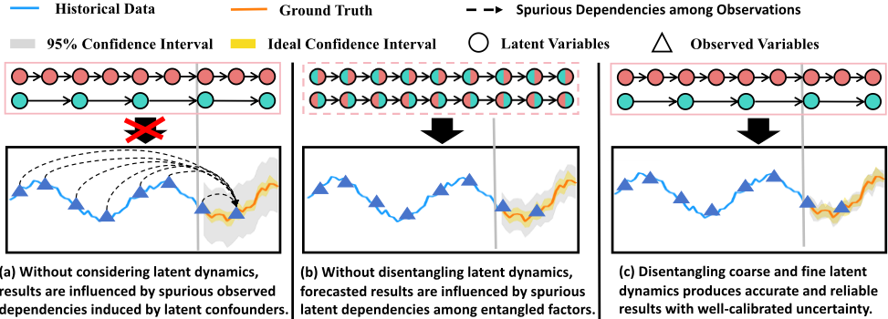
To tackle the challenge of probabilistic time series forecasting, researchers have proposed a range of methods. Previous methods directly extend the deterministic forecasting methods to the probabilistic forecasting setting. For instance, Salinas et al. [Salinas et al., 2020] presented DeepAR, an autoregressive RNN for probabilistic forecasting. Additionally, other methods model the uncertainty of historical observational variables to generate probabilistic forecasts. Li et al. [Li et al., 2022] utilize coupled diffusion processes and multi-scale denoising score matching to better approximate the true data distribution. And Marcel et al. [Kollovieh et al., 2023] proposed TSDiff, incorporating a self-guidance mechanism to adapt unconditional diffusion models for forecasting tasks. However, these methods directly model the uncertainty of observed variables while ignoring the underlying latent dynamics. As illustrated in Figure 1 (a), when the observed variables are influenced by unmodeled latent variables, these latent variables act as latent confounders. Consequently, the future observations become spuriously dependent on all historical observations, introducing excessive variability into the predictive distribution and finally resulting in overly wide confidence intervals.

Another group of methods considers the importance of latent dynamics. For instance, Tang et al. [Tang and Matteson, 2021] developed ProTran, leveraging attention mechanisms to capture non-Markovian dynamics for long-term forecasting. And Rasul et al. [Rasul et al., 2021b] introduced Transformer-MAF, which combines autoregressive flows with conditional regularization. Although existing methods have improved probabilistic forecasting by considering latent dynamics, they often overlook the complex mixture of latent dynamics. In many real-world systems, such as weather forecasting, observed variables are driven by coarse and fine latent factors, where coarse dynamics capture slow seasonal trends and fine dynamics reflect rapid daily fluctuations. Ignoring such coarse and fine latent dynamics can cause models to conflate distinct temporal structures, resulting in exaggerated fluctuations and unreliable uncertainty estimates. To illustrate this issue, consider the time-series data driven by latent dynamics at both coarse (green) and fine (pink) granularities in Figure 1. The coarse-scale dynamics (green circles) capture slow variations, whereas the fine-scale dynamics (pink circles) describe rapid and transient changes. However, as shown in Figure 1(b), when coarse and fine latent dynamics are entangled, the estimation of coarse dynamics tends to model excessive transitions that actually belong to the fine-scale dynamics. This over-transitioning introduces additional noise into the latent space, which is reflected in the variability of observed variables, ultimately inflating predictive uncertainty and widening the confidence intervals.

The above example underscores the necessity of accurately disentangling latent dynamics across different temporal scales and explicitly modeling how each latent process influences the observed variables. As illustrated in Figure 1(c), when coarse- and fine-scale latent information is properly disentangled, the model can effectively distinguish different types of variations, leading to smoother predictions and well-calibrated confidence intervals that align closely with the ideal one. Building on this insight, we introduce COFE (COarse and FinE latent dynamics disentanglement), a variational autoencoder-based framework explicitly designed to capture the coarse and fine latent dynamics underlying timeseries data. Rather than modeling temporal evolution at a single rate, COFE infers latent variables that evolve at distinct temporal scales, thereby providing a more faithful characterization of the observed data distribution. Importantly, our theoretical analysis establishes the block-wise identifiability of the coarse- and fine-grained latent variables, offering a principled foundation for disentangling multi-scale latent dynamics. This identifiability ensures that the model can independently capture slow and fast variations, avoiding redundant latent transitions that distort predictive uncertainty, and thus yielding sharper forecasts with better-calibrated confidence intervals. Extensive experiments further confirm that COFE achieves superior uncertainty quantification and consistently improves both accuracy and reliability across diverse real-world scenarios.

2 Preliminaries

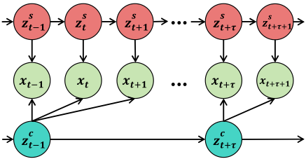
We begin with the generation process of the original timeseries data shown in Figure 2. The time series data with discrete time steps X = [x1, · · · , xT ] ∈ RT×d , Where d denotes the dimension of variable. We define zs = [zs1 , · · · , zsT ] ∈ RT×ns as the sequence of fine-grain latent variable, and zc = [zc1 , · · · , zcT ] ∈ RT×nc as the sequence of coarse-grain latent variable. Supposed that each moment the observed variables xt are generated by zst and zct through a nonlinear mixing process g as shown in Equation(1).

Formula not decoded

At time t, both the i-th dimension of latent variables zst and zct are generated by a latent causal process. This process assumes that latent variables are associated with their corresponding delayed parent nodes, as detailed in the following formula:

Formula not decoded

where ϵst,i , ϵct,i respectively signifies temporally and spatially independent noise drawn from the distribution pϵst,i and pϵct,i .

Based on the aforementioned description of the data generation process, probabilistic time series forecasting is fundamentally a conditional generative task. Given a historical sequence up to time L: X1:L = [x1, · · · , xL] ∈ RL×d , the objective is to model the conditional distribution P(XL+1:H|X1:L). We denote X1:L as the context and XL+1:H as the target.

3 Approach

This section elaborates on the implementation of the proposed COFE model illustrated in Figure 3. Specifically, the model adopts a variational sequential autoencoder to model the time series data. Moreover, we further leverage the independent noise estimator to model the latent dynamics and a sparse transition constraint to disentangle the latent dynamics of different scales.

3.1 Variational Inference-Based Time Series Modeling

We model the data generation process through variational inference, thereby deriving the ELBO show in the Equation 3.

Formula not decoded

The first component of ELBO is divided into reconstruction and prediction loss, denoted by LR and Ly, respectively. The corresponding formulas are as follows:

Formula not decoded

DKL indicates the KL divergence. The posterior distribution q(zs1:H |x1:H), q(zc1:H |x1:H) contains the encoder and the latent variable predictor module in Figure 3 and they need to match the prior distribution p(zs1:H ), p(zc1:H ), namely the standard normal distribution. p(x1:H|zs1:H , zc1:H ) denotes the process of reconstructing observed variables and predicting the distribution of future values. Express the two distributions mentioned above using the following formula:

Formula not decoded

where ϕ and ψ represent the encoder and decoder, respectively. And ˆz1:H denotes the combination of ˆzs1:H and ˆzc1:H . For the implementation of the encoder and decoder, we primarily adopted a structure based on MLP (Multi-Layer Perceptron). We provide more specific implementation details of the model in Appendix B.2.

3.2 Independent Noise Estimator

To model the latent variables with different scales and the prior distribution, we propose a prior network. Similar to existing causal representation learning methods, let rs i be a set of learned inverse transition functions, where the input is By using the change of variables formula, we have:

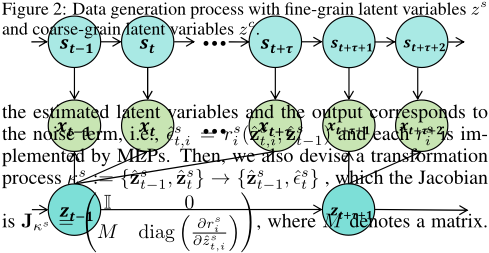
Figure 1: Illustration of how disentangling coarse and fine latent dynamics improves probabilistic time-series forecasting. (a) Without modeling latent dynamics, observed variables exhibit spurious dependencies induced by latent confounders, leading to inflated predictive uncertainty. (b) When latent dynamics are modeled but remain entangled, spurious dependencies persist among latent factors. (c) Properly disentangling coarse and fine latent dynamics enables the model to produce accurate and reliable results with well-calibrated uncertainty. (Best viewed in color.)

Formula not decoded

Since the noise term in Equation (6) is assumed independent of ˆzst-1 , we can enforce the independence of the estimated noise ˆ ϵst , with the following further result:

Formula not decoded

Therefore, the prior for the estimated latent variable ˆzs can be estimated using the following formula:

Formula not decoded

where p(ˆ ϵst ) satisfies Gaussian distribution. Similarly, the prior of the latent variable ˆzc can be evaluated using the following formula:

Formula not decoded

3.3 Sparse Transition Constraint

To disentangle the latent variables, we propose the sparse transition constraint. Latent variables zc exhibit deterministic processes where the noise term is zero. Latent variable zs incorporates noise at every time step. Based on this intuition, constraints on the rate of change of latent variables can be transformed into sparsity constraints on the corresponding noise sequences. We consider learning the noise sequence of the latent variable sequence through the aforementioned independent noise estimator:

Formula not decoded

where rs is the set of rs t,i , t ∈ 1, 2, ...,H -1 and i ∈ 1, 2, ..., ns, the same applies to rc . After obtaining the latent variable noise sequence, To measure the sparsity of noise sequences, we employ a smoothing approximation method based on the sigmoid function, as shown in Equation (11).

Formula not decoded

Figure 3: The complete framework of the proposed COFE model comprises an encoder for extracting latent variables ˆ zs 1:L and ˆ zc 1:L, a decoder for reconstructing observed variables ˆx1:L, a transition module for estimating ˆ zsL+1:H and ˆ zcL+1:H, a distribution predictor, and an estimator for adjacent latent state transition noise.

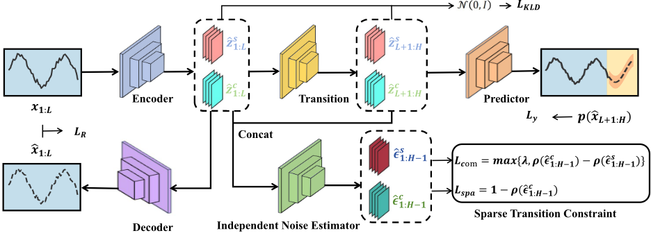
where σ(·) is the sigmoid function. δ is a threshold value, when the noise value falls below this threshold, it is treated as zero. For latent variable zc , its noise sequence should be sparse, with higher frequencies corresponding to greater sparsity. We aim to constrain the noise sequence associated with one of the learned latent variables to be as sparse as possible, that is, to maximize the value of ρ(ˆ ϵc1:H-1 ). Based on this intuition, we designed the loss function shown in Equation (12).

Formula not decoded

To enable the model to effectively learn latent variables zs and zc , constraints must be imposed on the relationship between their respective noise sequences: specifically, the sparsity of the noise sequence corresponding to the latent variable zs should be lower than that of the latent variable zc . The corresponding loss is as shown in the Equation (13).

Formula not decoded

where λ is a constant.

3.4 Model Summary

By combining the variational sequential autoencoder design described above with two types of regularization loss terms, which are proposed in 3.3, the overall loss function for the proposed COFE model are shown as follows:

Formula not decoded

where α, β, γ, and η are hyperparameters.

4 Theoretical Analysis

We further establish the identification theory for the disentanglement guarantees between zst and zct . We first provide the definition of block-wise identification in Definition 1.

Definition 1 (Block-wise Identifiability of Latent Variables). The block-wise identifiability of z ∈ Rnd means that for ground-truth z, there exists ˆz and an invertible function h : Rnd → Rnd , such that z = h(ˆz).

Theorem1. (Block-wise Identification of the latent variable zst and zct ) We assume the data generation process following Figure 2 and further make the following assumptions:

A1 (Smooth, Positive Density:) [Yao et al., 2022; Kong et al., 2022; Yao et al., 2021] The probability density function of latent variables is smooth and positive, i.e., p(zst |zst-1 ) > 0 over zst-1 and zst .
A2 (Conditional independent): [Yao et al., 2022; Yao et al., 2021] Conditioned on u = zst-1 each zst,i is independent of any other zst,j for i, j ∈ 1, ..., n, i ̸= j, i.e, log p(zst |u) = ∑ns 1 log p(zt,i|u)
A3 (Linear Independence:) [Yao et al., 2022; Li et al., 2024b] For any zst ⊆ Rns , there exist ns + 1 values of u = zst-1 , i.e., us with j = 0, 1, ..., ns, such that these ns vectors v(zs , uj )-v(zs , u0) with j = 1, ..., ns are linearly independent, Where v(zs , uj) are formalized as follows:

Formula not decoded

Suppose that the learned (ˆ g, ˆ f , pˆ ϵ) satisfies Equation (1)- (3), then the latent variable zst and zct are block-wise identifiable.

Proof Sketch: The complete proof process can be found in Appendix B. The intuition and explanation of the assumptions are shown in Appendix B.3. The theory demonstrates that zst and zct can be identified through a fixed set of observations. Due to variations in latent variable frequencies, different causal structures may emerge during the proof process. However, after discussion, all can be traced back to proving the same structure. First, we establish an invertible transformation process h between the true latent variable and the estimated one. Then, we construct a linear full-rank system as shown in Equation (16) using variables from different domains, where the unique solution is ∂zst ∂ˆzct = 0 .

Table 1: Experimental results on short-term datasets. Bold numbers indicate the best results, and underlined numbers indicate the second-best results.
Model	Metric	Exchange-S	Solar-S	Electricity-S	ETTh1-S	ETTh2-S	ETTm1-S	ETTm2-S	Mean
FITS	CRPS NMAE	0.012± 0.002 0.017± 0.003	0.516± 0.011 0.701± 0.014	0.068± 0.003 0.092±	0.320± 0.017 0.423± 0.033	0.212± 0.012 0.278± 0.009	0.193± 0.005 0.249± 0.007	0.199± 0.003 0.260± 0.011	0.217 0.289
	CRPS	0.052± 0.016	0.491± 0.008	0.004 0.063± 0.003	0.314± 0.022	0.207± 0.006	0.234± 0.011	0.212± 0.018 0.257± 0.011	0.225 0.287
PatchTST	NMAE	0.069± 0.013	0.663± 0.010	0.085± 0.006	0.407± 0.030	0.260± 0.009	0.271± 0.009
iTransformer	CRPS	0.059± 0.018	0.504± 0.012	0.066± 0.004	0.317± 0.020	0.219± 0.008	0.254± 0.012	0.201± 0.018	0.231
	NMAE	0.081± 0.022				0.276± 0.017	0.291± 0.017	0.242± 0.009
			0.695± 0.017	0.087± 0.006	0.408± 0.028				0.297
Koopa	CRPS	0.012± 0.001	0.545± 0.016	0.085± 0.014	0.326± 0.013	0.211± 0.019	0.288± 0.022	0.220± 0.015	0.241
	NMAE	0.015± 0.002	0.742± 0.022	0.112± 0.019	0.423± 0.017	0.266± 0.022	0.329± 0.026	0.278± 0.022	0.309
	CRPS	0.019	0.568± 0.015	0.111± 0.013	0.304± 0.016	0.204± 0.006	0.209± 0.013	0.124± 0.008	0.228
TSDiff	NMAE	0.077± 0.096± 0.024	0.635± 0.012	0.115± 0.018	0.400± 0.025	0.272± 0.015	0.276± 0.008	0.162± 0.008	0.279
D3VAE	CRPS NMAE	0.011 ± 0.002 0.012 ± 0.002	0.769± 0.029 0.998± 0.049	0.071± 0.009 0.092± 0.013	0.324± 0.019 0.410± 0.016	0.216± 0.015 0.267± 0.018	0.198± 0.015 0.250± 0.018	0.303± 0.024 0.378± 0.031	0.270 0.344
	CRPS NMAE	0.019± 0.006 0.024± 0.007	0.530± 0.008 0.670± 0.011	0.062± 0.003 0.081± 0.006	0.398± 0.034 0.477± 0.040	0.309± 0.023 0.375± 0.024	0.455± 0.029 0.584± 0.047	0.276± 0.014 0.349± 0.028	0.293 0.365
GRUNVP		0.012± 0.003	0.486± 0.007			0.008	0.009	0.146± 0.011	0.181
GRUMAF	CRPS	0.016± 0.002		0.056± 0.002	0.258± 0.013	0.160± 0.208± 0.003	0.151± 0.004	0.193± 0.008	0.231
	NMAE CRPS	0.012± 0.001	0.603± 0.009 0.442± 0.011	0.073± 0.004 0.054± 0.002	0.326± 0.016 0.309± 0.009	0.200± 0.012	0.198± 0.139± 0.005	0.180± 0.010	0.191
Trans MAF	NMAE	0.016± 0.001	0.577± 0.014	0.071± 0.003	0.400± 0.011	0.256± 0.009	0.162± 0.006	0.224± 0.009	0.244
TimeGrad	CRPS	0.009± 0.001	0.465± 0.016	0.057± 0.002	0.273± 0.007	0.184± 0.006	0.186± 0.003	0.148± 0.004	0.189
	NMAE	0.012 ± 0.002	0.609± 0.015	0.073± 0.004	0.356± 0.013	0.224± 0.014	0.246± 0.007	0.189± 0.006	0.244
CSDI	CRPS	0.009± 0.001	0.392± 0.006	0.051± 0.001	0.262± 0.012	0.133± 0.006	0.012	0.144± 0.018	0.162
	NMAE	0.013± 0.001	0.533± 0.007	0.066± 0.001	0.339± 0.009	0.161± 0.013	0.140± 0.169± 0.021	0.181± 0.024	0.209
K2VAE	CRPS	0.009± 0.001	0.367 ± 0.005	0.053 ± 0.002	0.256 ± 0.008	0.128 ± 0.006	0.135 ± 0.008	0.122 ± 0.008	0.153
	NMAE	0.009± 0.001 0.009± 0.0002	0.480 ± 0.008	0.068 ± 0.002	0.312 ± 0.008	0.140 ± 0.007 0.119±	0.152 ± 0.007 0.002	0.146 ± 0.009 0.113± 0.001	0.187
COFE	CRPS NMAE		0.362± 0.001	0.053 ± 0.001	0.251± 0.004 0.005	0.002	0.119±		0.147
		0.009± 0.0001	0.459± 0.004	0.068 ± 0.001	0.306±	0.137± 0.003	0.132± 0.003	0.136± 0.002	0.178

Formula not decoded

Implication of theoretical results: This theorem provides the theoretical foundation for disentangling coarse-grained and fine-grained latent variables in time series data. In probabilistic time series forecasting, this is essential for improving both accuracy and uncertainty estimation. By proving that the latent variables zst and zct are block-wise identifiable, the theory ensures that the model can separately capture slow, largescale trends and fast, local variations. This separation avoids mixing latent dependencies that often lead to inflated uncertainty, enabling the model to generate sharper forecasts and well-calibrated confidence intervals. In practice, this guarantees that the probabilistic predictions reflect the true multiscale structure of real-world temporal data.

5 Experiments

5.1 Datasets

We consider the following datasets. ETT dataset comprises electrical transformer temperature data collected from two distinct counties in China. Exchange 1 dataset contains daily exchange rate data from eight foreign countries, with a time span from 1990 to 2016. Solar 2 dataset Contains solar power generation records from 2006, sampled every 10 minutes from 137 photovoltaic power stations in Alabama. Electricity 3 dataset includes power consumption from 321 clients between 2012 and 2014. ILI [Wu et al., 2021] dataset includes the ratio of patients with influenza-like illness and the number of patients per week in the United States from 2002 to 2021. Weather 4 dataset includes 21 meteorological indicators mearesults.

1 https://data.imf.org/en/datasets/IMF.STA:ER

2 https://zenodo.org/records/3889974

Figure 4: Model efficiency comparison. All data is statistics from ETTm1-S, including inference efficiency and the maximum GPU memory usage during one epoch. A lower CRPS value indicates better model performance.

3 https://pacificdata.org/data/dataset/ tuvalu-electricity-corporation-electricity-statistics-2012-2014

4 https://www.kaggle.com/datasets/alistairking/ weather-long-term-time-series-forecasting

Model	Metric	ETTm1-L	ETTm2-L	ETTh1-L	ETTh2-L	Electricity-L	Weather-L	Exchange-L	ILI-L	Mean
FITS	CRPS NMAE	0.305± 0.024 0.406± 0.072	0.449± 0.034 0.540± 0.052	0.348± 0.025 0.468± 0.012	0.314± 0.022 0.401± 0.022	0.115± 0.024 0.149± 0.012	0.267± 0.003 0.317± 0.021	0.074± 0.011 0.097± 0.011	0.211± 0.011 0.245± 0.017	0.260 0.328
PatchTST	CRPS NMAE	0.304± 0.029 0.382± 0.066	0.229± 0.036 0.288± 0.034	0.323± 0.020 0.428± 0.024	0.304± 0.018 0.371± 0.021	0.127± 0.015 0.164± 0.024	0.142± 0.005 0.152± 0.029	0.097± 0.007 0.126± 0.001	0.233± 0.019 0.287± 0.023	0.220 0.275
iTransformer	CRPS NMAE	0.455± 0.021 0.490± 0.038	0.311± 0.024 0.385± 0.042	0.350± 0.019 0.449± 0.022	0.542± 0.015 0.667± 0.012	0.109± 0.044 0.140± 0.009	0.133± 0.004 0.147± 0.019	0.087± 0.023 0.113± 0.015	0.222± 0.020 0.278± 0.017	0.276 0.334
Koopa	CRPS NMAE	0.295± 0.027 0.377± 0.037	0.233± 0.025 0.290± 0.033	0.318± 0.009 0.412± 0.008	0.293± 0.026 0.286± 0.042	0.113± 0.018 0.149± 0.025	0.140± 0.007 0.162± 0.009	0.091± 0.012 0.116± 0.022	0.228± 0.022 0.288± 0.031	0.214 0.260
TSDiff	CRPS NMAE	0.478± 0.027 0.622± 0.045	0.344± 0.046 0.416± 0.065	0.516± 0.027 0.657± 0.017	0.406± 0.056 0.482± 0.022	0.478± 0.005 0.622± 0.142	0.152± 0.003 0.141± 0.026	0.082± 0.010 0.142± 0.009	0.263± 0.022 0.272± 0.020	0.340 0.419
GRUNVP	CRPS NMAE	0.546± 0.036 0.707± 0.050	0.561± 0.273 0.749± 0.385	0.502± 0.039 0.643± 0.046	0.539± 0.090 0.688± 0.161	0.114± 0.013 0.144± 0.017	0.110± 0.004 0.135± 0.008	0.079± 0.009 0.103± 0.009	0.307± 0.005 0.333± 0.005	0.345 0.437
GRUMAF	CRPS NMAE	0.536± 0.033 0.711± 0.081	0.272± 0.029 0.355± 0.048	0.393± 0.043 0.496± 0.019	0.990± 0.023 1.092± 0.019	0.106± 0.007 0.136± 0.098	0.122± 0.006 0.149± 0.034	0.160± 0.019 0.182± 0.010	0.172± 0.034 0.216± 0.014	0.344 0.417
Trans MAF	CRPS NMAE	0.688± 0.043 0.822± 0.034	0.355± 0.043 0.475± 0.029	0.363± 0.053 0.455± 0.025	0.327± 0.033 0.412± 0.020	- -	0.113± 0.004 0.148± 0.040	0.148± 0.017 0.191± 0.006	0.155± 0.018 0.183± 0.019	- -
TimeGrad	CRPS NMAE CRPS	0.621± 0.037 0.793± 0.034 0.448± 0.038	0.470± 0.054 0.561± 0.044 0.239± 0.035	0.523± 0.027 0.672± 0.015 0.528± 0.012	0.445± 0.016 0.550± 0.018 0.040	0.108± 0.003 0.134± 0.004	0.113± 0.011 0.136± 0.020 0.087 ± 0.003	0.099± 0.015 0.113± 0.016 0.143± 0.020	0.295± 0.083 0.325± 0.068 0.283± 0.012	0.334 0.411 -
CSDI	NMAE CRPS	0.578± 0.051 0.294± 0.026	0.306± 0.040	0.657± 0.014	0.302± 0.382± 0.030	- -	0.102± 0.005	0.173± 0.020	0.299± 0.013	- 0.183
K2VAE	NMAE	0.373± 0.032	0.221 ± 0.023 0.275 ± 0.035	0.314 ± 0.011 0.396 ± 0.012	0.280 ± 0.014 0.278 ± 0.020	0.057± 0.005 0.117± 0.019	0.084± 0.003 0.099 ± 0.009	0.069 ± 0.005 0.084 ± 0.017	0.142 ± 0.008 0.167 ± 0.007	0.224
COFE	CRPS NMAE	0.289± 0.004 0.368± 0.005	0.207± 0.003 0.235± 0.001	0.304± 0.002 0.390± 0.005	0.218± 0.017 0.251± 0.008	0.105± 0.001 0.129± 0.002	0.092± 0.001 0.001	0.066± 0.001	0.119± 0.003 0.154± 0.004	0.175 0.213
Table 2:	Experimental	results on	long-term datasets.	Bold numbers	indicate	the best results,	0.097± and underlined	0.079± 0.005 numbers	indicate the	second-best

Figure 5: Ablation study on the ETTm1-S and ILI-L datasets.

sured every 10 minutes. More details about the datasets are provided in Appendix C.1. For each dataset, we follow the standard preprocessing procedures and experimental configurations established in ProbTS [Zhang et al., 2024a].

5.2 Baselines

We compared COFE with a total of 12 outstanding baselines. We consider eight state-of-the-art probabilistic forecasting models: K2VAE [Wu et al., 2025], TSDiff [Kollovieh et al., 2023], D3VAE [Li et al., 2022], GRU NVP, GRU MAF, Trans MAF[Rasul et al., 2021b], TimeGrad [Rasul et al., 2021a], and CSDI [Tashiro et al., 2021], in the shortand long-term probabilistic prediction scenarios proposed by ProbTS [Zhang et al., 2024a]. we also consider four point forecasting models: FITS [Xu et al., 2024], PatchTST [Nie et al., 2022], iTransformer [Liu et al., 2023a] and Koopa [Liu et al., 2023b].

5.3 EvaluationMetric

To assess the probabilistic forecasts, we employ two widely adopted metrics: CRPS (Continuous Ranked Probability Score) and NMAE (Normalized Mean Absolute Error). More details are provided in appendix C.2.

5.4 Main Results and Discussion

Experimental results on short- and long-term datasets are presented in Table 1 and Table 2. Since some methods report the mean and standard deviation of results, we also show the mean and standard deviation of our results after five independent runs. Notably, the proposed COFE model achieves significantly optimized results compared to baseline methods on most datasets. However, our model achieved suboptimal yet still competitive results on the Electricity dataset, which may be due to its high dimensionality making the identification of latent variables challenging. To further demonstrate the performance of the COFE model, we also conducted Ablation experiments and visualizations. Compared to other models, our proposed model not only demonstrates the best performance but also exhibits excellent model efficiency. More experimental details are provided in appendix C.3.

5.5 Ablation Studies

We designed a series of variants of the COFE model to validate the effectiveness of the proposed components. 1) COFEKLD: Removed the Kullback-Leibler divergence term. 2) COFE-com: Removed the constraint on the speed difference between different latent variables 3) COFE-spa: Removed sparse constraints on noise sequences for coarse latent variable 4) COFE-R: Removed the constraints on reconstructing observation. Experiment results of the ablation studies on the ETTm1-S and ILI-L datasets are shown in Figure 5. The results indicate that all loss terms play crucial roles. Removing the KL divergence term significantly degrades model performance, as it enhances the distinguishability of latent variables in the relevant latent space. Notably, the performance of COFE-R, COFE-spa, and COFE-com deteriorates, demonstrating that the reconstruction loss helps preserve information in observed variables. Furthermore, our constraints enable the model to learn coarse and fine latent dynamics, validating the effectiveness of our approach.

Figure 6: Visualization of probabilistic forecasting results on the ETTm1-S and ILI-L datasets. Our method produces more reasonable confidence intervals and mean predictions that more closely follow the ground truth observations.

5.6 Visualization Results

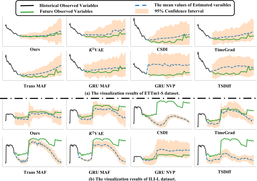
We further provide visualizations of results on the ETTm1-S and ILI-L datasets in Figure 6. Notably, compared to baselines, our approach achieves more efficient and compact confidence interval estimation. This demonstrates that the model avoids both under-coverage due to overly narrow confidence intervals and redundancy caused by excessively wide intervals when quantifying uncertainty. This is because the COFE model decouples and fully captures coarse and fine dynamics, thereby more accurately characterizing the conditional distribution of future observations.

5.7 Model Efficiency

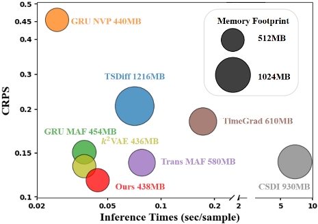
We evaluate the efficiency of the model in three dimensions: predictive performance (CRPS), inference efficiency, and maximum GPU memory usage, as shown in Figure 4. Our approach achieves optimal predictive performance while utilizing minimal GPU memory and achieving fast inference speed, demonstrating high efficiency. This is due to the model's architecture, which is primarily constructed using MLP or linear layers, enabling efficient extraction of latent variables and generation of predictions.We further conducted a sensitivity analysis on the key hyperparameters of the model, presented in Appendix D.

6 Summary

This paper introduces a principled framework for probabilistic time series forecasting that explicitly disentangles and models coarse and fine latent dynamics. The key insight is that observed uncertainty arises from latent processes evolving at different transition speeds, such as slow seasonal and fast daily variations in climate data. To achieve this, the proposed COFE framework leverages a variational autoencoder with an independent transition noise estimation module and a sparsity constraint to disentangle latent dynamics across scales. Theoretically, COFE ensures block-wise identifiability of the coarse and fine latent dynamics, and empirically, it achieves superior forecasting accuracy and sharper uncertainty quantification across 15 benchmark datasets.

Changze Zhou, Ruichu Cai, Shengbin Nie, Juntao Fang, Jie Qiao, and Zijian Li. 2026. Disentangling Coarse and Fine Latent Dynamics for Probabilistic Time Series Forecasting. In Proceedings of the Thirty-Fifth International Joint Conference on Artificial Intelligence, IJCAI-26. IJCAI, 5404–5412. https://doi.org/10.24963/ijcai.2026/602

@inproceedings{ijcai2026p602,
  title     = {Disentangling Coarse and Fine Latent Dynamics for Probabilistic Time Series Forecasting},
  author    = {Zhou, Changze and Cai, Ruichu and Nie, Shengbin and Fang, Juntao and Qiao, Jie and Li, Zijian},
  booktitle = {Proceedings of the Thirty-Fifth International Joint Conference on
               Artificial Intelligence, {IJCAI-26}},
  publisher = {International Joint Conferences on Artificial Intelligence Organization},
  editor    = {Diego Calvanese},
  pages     = {5404--5412},
  year      = {2026},
  month     = {8},
  note      = {Main Track},
  doi       = {10.24963/ijcai.2026/602},
  url       = {https://doi.org/10.24963/ijcai.2026/602},
}

TY  - CPAPER
TI  - Disentangling Coarse and Fine Latent Dynamics for Probabilistic Time Series Forecasting
AU  - Zhou, Changze
AU  - Cai, Ruichu
AU  - Nie, Shengbin
AU  - Fang, Juntao
AU  - Qiao, Jie
AU  - Li, Zijian
T2  - Proceedings of the Thirty-Fifth International Joint Conference on Artificial Intelligence, IJCAI-26
PB  - International Joint Conferences on Artificial Intelligence Organization
PY  - 2026
SP  - 5404
EP  - 5412
DO  - 10.24963/ijcai.2026/602
UR  - https://doi.org/10.24963/ijcai.2026/602
ER  -

[1] [Bacanin et al., 2023] Nebojsa Bacanin, Luka Jovanovic, Miodrag Zivkovic, Venkatachalam Kandasamy, Milos An- tonijevic, Muhammet Deveci, and Ivana Strumberger. Multivariate energy forecasting via metaheuristic tuned long-short term memory and gated recurrent unit neural networks. Information Sciences, 642:119122, 2023.

[2] [Bergsma et al., 2022] Shane Bergsma, Tim Zeyl, Javad Rahimipour Anaraki, and Lei Guo. C2far: Coarse-to-fine autoregressive networks for precise probabilistic forecast- ing. Advances in Neural Information Processing Systems, 35:21900-21915, 2022.

[3] [Daunhawer et al., 2023] Imant Daunhawer, Alice Bizeul, Emanuele Palumbo, Alexander Marx, and Julia E Vogt. Identifiability results for multimodal contrastive learning. arXiv preprint arXiv:2303.09166, 2023.

[4] [Hyvarinen and Morioka, 2016] Aapo Hyvarinen and Hi- roshi Morioka. Unsupervised feature extraction by time- contrastive learning and nonlinear ica. Advances in neural information processing systems, 29, 2016.

[5] [Hyvärinen and Pajunen, 1999] Aapo Hyvärinen and Petteri Pajunen. Nonlinear independent component analysis: Existence and uniqueness results. Neural networks, 12(3):429-439, 1999.

[6] [Jhin et al., 2024] Sheo Yon Jhin, Seojin Kim, and Noseong Park. Addressing prediction delays in time series forecast- ing: A continuous gru approach with derivative regular- ization. In Proceedings of the 30th ACM SIGKDD Con- ference on Knowledge Discovery and Data Mining, KDD '24, page 1234-1245, New York, NY, USA, 2024. Associ- ation for Computing Machinery.

[7] [Khemakhem et al., 2020] Ilyes Khemakhem, Diederik Kingma, Ricardo Monti, and Aapo Hyvarinen. Variational autoencoders and nonlinear ica: A unifying framework. In International conference on artificial intelligence and statistics, pages 2207-2217. PMLR, 2020.

[8] [Kollovieh et al., 2023] Marcel Kollovieh, Abdul Fatir Ansari, Michael Bohlke-Schneider, Jasper Zschiegner, Hao Wang, and Yuyang Bernie Wang. Predict, refine, synthesize: Self-guiding diffusion models for probabilistic time series forecasting. Advances in Neural Information Processing Systems, 36:28341-28364, 2023.

[9] [Kollovieh et al., 2024] Marcel Kollovieh, Marten Lienen, David Lüdke, Leo Schwinn, and Stephan Günnemann. Flow matching with gaussian process priors for prob- abilistic time series forecasting. arXiv preprint arXiv:2410.03024, 2024.

[10] [Kong et al., 2022] Lingjing Kong, Shaoan Xie, Weiran Yao, Yujia Zheng, Guangyi Chen, Petar Stojanov, Victor Akin- wande, and Kun Zhang. Partial disentanglement for do- main adaptation. In International conference on machine learning, pages 11455-11472. PMLR, 2022.

[11] [Lachapelle et al., 2023] Sébastien Lachapelle, Tristan Deleu, Divyat Mahajan, Ioannis Mitliagkas, Yoshua Bengio, Simon Lacoste-Julien, and Quentin Bertrand. Synergies between disentanglement and sparsity: Gen- eralization and identifiability in multi-task learning. In International Conference on Machine Learning, pages 18171-18206. PMLR, 2023.

[12] [Lai et al., 2018] Guokun Lai, Wei-Cheng Chang, Yiming Yang, and Hanxiao Liu. Modeling long-and short-term temporal patterns with deep neural networks. In The 41st international ACM SIGIR conference on research & devel- opment in information retrieval, pages 95-104, 2018.

[13] [Li et al., 2022] Yan Li, Xinjiang Lu, Yaqing Wang, and De- jing Dou. Generative time series forecasting with diffu- sion, denoise, and disentanglement. Advances in Neural Information Processing Systems, 35:23009-23022, 2022.

[14] [Li et al., 2024a] Yuxin Li, Wenchao Chen, Xinyue Hu, Bo Chen, Mingyuan Zhou, et al. Transformer-modulated diffusion models for probabilistic multivariate time series forecasting. In The Twelfth International Conference on Learning Representations, 2024.

[15] [Li et al., 2024b] Zijian Li, Yifan Shen, Kaitao Zheng, Ruichu Cai, Xiangchen Song, Mingming Gong, Zheng- mao Zhu, Guangyi Chen, and Kun Zhang. On the iden- tification of temporally causal representation with instan- taneous dependence. arXiv preprint arXiv:2405.15325, 2024.

[16] [Li et al., 2025] Qi Li, Zhenyu Zhang, Lei Yao, Zhaoxia Li, Tianyi Zhong, and Yong Zhang. Diffusion-based decou- pled deterministic and uncertain framework for proba- bilistic multivariate time series forecasting. In The Thir- teenth International Conference on Learning Representa- tions, 2025.

[17] [Lippi et al., 2013] Marco Lippi, Matteo Bertini, and Paolo Frasconi. Short-term traffic flow forecasting: An experi- mental comparison of time-series analysis and supervised learning. IEEE Transactions on Intelligent Transportation Systems, 14(2):871-882, 2013.

[18] [Liu et al., 2023a] Yong Liu, Tengge Hu, Haoran Zhang, Haixu Wu, Shiyu Wang, Lintao Ma, and Mingsheng Long. itransformer: Inverted transformers are effective for time series forecasting. arXiv preprint arXiv:2310.06625, 2023.

[19] [Liu et al., 2023b] Yong Liu, Chenyu Li, Jianmin Wang, and Mingsheng Long. Koopa: learning non-stationary time series dynamics with koopman predictors. In Proceedings of the 37th International Conference on Neural Informa- tion Processing Systems, NIPS '23, Red Hook, NY, USA, 2023.

[20] Curran Associates Inc. [Nguyen and Quanz, 2021] Nam Nguyen and Brian Quanz. Temporal latent auto-encoder: A method for probabilis- tic multivariate time series forecasting. In Proceedings of the AAAI conference on artificial intelligence, volume 35, pages 9117-9125, 2021.

[21] [Nie et al., 2022] Yuqi Nie, Nam H Nguyen, Phanwadee Sinthong, and Jayant Kalagnanam. A time series is worth 64 words: Long-term forecasting with transformers. arXiv preprint arXiv:2211.14730, 2022.

[22] [Rasul et al., 2021a] Kashif Rasul, Calvin Seward, Ingmar Schuster, and Roland Vollgraf. Autoregressive denoising diffusion models for multivariate probabilistic time series forecasting. In International conference on machine learn- ing, pages 8857-8868. PMLR, 2021.

[23] [Rasul et al., 2021b] Kashif Rasul, Abdul-Saboor Sheikh, Ingmar Schuster, Urs M Bergmann, and Roland Vollgraf. Multivariate probabilistic time series forecasting via con- ditioned normalizing flows. In International Conference on Learning Representations, 2021.

[24] [Salinas et al., 2020] David Salinas, Valentin Flunkert, Jan Gasthaus, and Tim Januschowski. Deepar: Probabilistic forecasting with autoregressive recurrent networks. Inter- national journal of forecasting, 36(3):1181-1191, 2020.

[25] [Sezer et al., 2020] Omer Berat Sezer, Mehmet Ugur Gudelek, and Ahmet Murat Ozbayoglu. Financial time series forecasting with deep learning: A systematic literature review: 2005-2019. Applied soft computing, 90:106181, 2020.

[26] [Si et al., 2025] Haotian Si, Changhua Pei, Jianhui li, Dan Pei, and Gaogang Xie. CMos: Rethinking time series prediction through the lens of chunk-wise spatial corre- lations. In Forty-second International Conference on Ma- chine Learning, 2025.

[27] [Song et al., 2023] Xiangchen Song, Weiran Yao, Yewen Fan, Xinshuai Dong, Guangyi Chen, Juan Carlos Niebles, Eric Xing, and Kun Zhang. Temporally disentan- gled representation learning under unknown nonstationar- ity. Advances in Neural Information Processing Systems, 36:8092-8113, 2023.

[28] [Tang and Matteson, 2021] Binh Tang and David S Matte- son. Probabilistic transformer for time series analy- sis. Advances in neural information processing systems, 34:23592-23608, 2021.

[29] [Tashiro et al., 2021] Yusuke Tashiro, Jiaming Song, Yang Song, and Stefano Ermon. Csdi: Conditional score- based diffusion models for probabilistic time series im- putation. Advances in neural information processing sys- tems, 34:24804-24816, 2021.

[30] [Wang et al., 2023] Xinyi Wang, Meijen Lee, Qing Zhao, and Lang Tong. Non-parametric probabilistic time series forecasting via innovations representation. arXiv preprint arXiv:2306.03782, 2023.

[31] [Wang et al., 2025] Yulong Wang, Yushuo Liu, Xiaoyi Duan, and Kai Wang. Filterts: Comprehensive frequency filtering for multivariate time series forecasting. Proceed- ings of the AAAI Conference on Artificial Intelligence, 39(20):21375-21383, Apr. 2025.

[32] [Wu et al., 2021] Haixu Wu, Jiehui Xu, Jianmin Wang, and Mingsheng Long. Autoformer: Decomposition transform- ers with auto-correlation for long-term series forecast- ing. Advances in neural information processing systems, 34:22419-22430, 2021.

[33] [Wu et al., 2022] Haixu Wu, Tengge Hu, Yong Liu, Hang Zhou, Jianmin Wang, and Mingsheng Long. Timesnet: Temporal 2d-variation modeling for general time series analysis. arXiv preprint arXiv:2210.02186, 2022.

[34] [Wu et al., 2025] Xingjian Wu, Xiangfei Qiu, Hongfan Gao, Jilin Hu, Bin Yang, and Chenjuan Guo. k 2 vae: A koopman-kalman enhanced variational autoencoder for probabilistic time series forecasting. arXiv preprint arXiv:2505.23017, 2025.

[35] [Xie et al., 2023] Shaoan Xie, Lingjing Kong, Mingming Gong, and Kun Zhang. Multi-domain image generation and translation with identifiability guarantees. In The Eleventh international conference on learning representa- tions, 2023.

[36] [Xu et al., 2024] Zhijian Xu, Ailing Zeng, and Qiang Xu. FITS: Modeling time series with $10k$ parameters. In The Twelfth International Conference on Learning Repre- sentations, 2024.

[37] [Yao et al., 2021] Weiran Yao, Yuewen Sun, Alex Ho, Changyin Sun, and Kun Zhang. Learning temporally causal latent processes from general temporal data. arXiv preprint arXiv:2110.05428, 2021.

[38] [Yao et al., 2022] Weiran Yao, Guangyi Chen, and Kun Zhang. Temporally disentangled representation learning. arXiv preprint arXiv:2210.13647, 2022.

[39] [Yao et al., 2023] Dingling Yao, Danru Xu, Sébastien Lachapelle, Sara Magliacane, Perouz Taslakian, Georg Martius, Julius von Kügelgen, and Francesco Locatello. Multi-view causal representation learning with partial ob- servability. arXiv preprint arXiv:2311.04056, 2023.

[40] [Ye et al., 2025] Weiwei Ye, Zhuopeng Xu, and Ning Gui. Non-stationary diffusion for probabilistic time series fore- casting. arXiv preprint arXiv:2505.04278, 2025.

[41] [Zeng et al., 2023] Ailing Zeng, Muxi Chen, Lei Zhang, and Qiang Xu. Are transformers effective for time series fore- casting? In Proceedings of the AAAI conference on artifi- cial intelligence, volume 37, pages 11121-11128, 2023.

[42] [Zhang et al., 2024a] Jiawen Zhang, Xumeng Wen, Zhenwei Zhang, Shun Zheng, Jia Li, and Jiang Bian. Probts: Bench- marking point and distributional forecasting across diverse prediction horizons. In A. Globerson, L. Mackey, D. Bel- grave, A. Fan, U. Paquet, J. Tomczak, and C. Zhang, edi- tors, Advances in Neural Information Processing Systems, volume 37, pages 48045-48082.

[43] Curran Associates, Inc., 2024.

[44] [Zhang et al., 2024b] Kun Zhang, Shaoan Xie, Ignavier Ng, and Yujia Zheng. Causal representation learning from multiple distributions: A general setting. arXiv preprint arXiv:2402.05052, 2024.

[45] [Zheng and Sun, 2024] Vincent Zhihao Zheng and Lijun Sun. Multivariate probabilistic time series forecasting with correlated errors. Advances in Neural Information Pro- cessing Systems, 37:54288-54329, 2024.