
A Parallel Framework for the Maximum Common Induced Subgraph Problem
Proceedings of the Thirty-Fifth International Joint Conference on Artificial Intelligence. Main Track. Pages 6370-6378.
https://doi.org/10.24963/ijcai.2026/709
Keywords
- Search: Heuristic search
- Search: Combinatorial search and optimisation
Abstract
Finding the maximum common induced subgraph (MCIS) between two graphs is a well-known NP-hard problem. While sequential MCIS algorithms have been extensively studied, parallel computing has emerged as an important direction for further performance enhancement with the advancement of computing resources. In this paper, we propose a parallel MCIS framework integrating a dynamic task decomposition method guided by search information and a novel pruning strategy based on shared information. The experimental results demonstrate that the algorithm enhanced by our framework achieves superior performance over both state-of-the-art sequential and existing parallel algorithms. Extensive results further demonstrate the wide scalability and generality of our framework, and the effectiveness of our strategies.
- [Akutsu and Tamura, 2012] Tatsuya Akutsu and Takeyuki Tamura. On the complexity of the maximum common subgraph problem for partial k-trees of bounded degree. In ISAAC, pages 146-155, 2012.
- [Bai et al., 2021] Yunsheng Bai, Derek Xu, Yizhou Sun, and Wei Wang. Glsearch: Maximum common subgraph de- tection via learning to search. In ICML, pages 588-598, 2021.
- [Brin and Page, 1998] Sergey Brin and Lawrence Page. The anatomy of a large-scale hypertextual web search engine. Computer Networks and ISDN Systems, 30(1-7):107-117, 1998.
- [Calabrese et al., 2026] Andrea Calabrese, Lorenzo Car- done, Salvatore Licata, Marco Porro, and Stefano Quer. Improving state-of-the-art vertex sorting algorithms to compute the maximum common induced subgraph. Jour- nal of Heuristics, 32(1):1, 2026.
- [Choi et al., 2012] Jaeun Choi, Yourim Yoon, and Byung-Ro Moon. An efficient genetic algorithm for subgraph isomor- phism. In GECCO, pages 361-368, 2012.
- [Dalke and Hastings, 2013] Andrew Dalke and Janna Hast- ings. Fmcs: a novel algorithm for the multiple mcs prob- lem. Journal of Cheminformatics, 5(Suppl 1):O6, 2013.
- [Damiand et al., 2011] Guillaume Damiand, Christine Sol- non, Colin De la Higuera, Jean-Christophe Janodet, and Émilie Samuel. Polynomial algorithms for subisomor- phism of nd open combinatorial maps. Computer Vision and Image Understanding, 115(7):996-1010, 2011.
- [Fuchs and Riesen, 2025] Mathias Fuchs and Kaspar Riesen. Fast approximate maximum common subgraph computa- tion. Pattern Recognition Letters, 190:66-72, 2025.
- [Hoffmann et al., 2017] Ruth Hoffmann, Ciaran McCreesh, and Craig Reilly. Between subgraph isomorphism and maximum common subgraph. In AAAI, pages 3907-3914, 2017.
- [Hoffmann et al., 2018] Ruth Hoffmann, Ciaran McCreesh, Samba Ndojh Ndiaye, Patrick Prosser, Craig Reilly, Chris- tine Solnon, and James Trimble. Observations from par- allelising three maximum common (connected) subgraph algorithms. In CPAIOR, pages 298-315, 2018.
- [Kothalawala et al., 2025] Buddhi W Kothalawala, Henning Koehler, and Qing Wang. Learning to bound for maximum common subgraph algorithms. In CP, pages 22-1, 2025.
- [Liu et al., 2020] Yanli Liu, Chu-Min Li, Hua Jiang, and Kun He. A learning based branch and bound for maxi- mum common subgraph related problems. In AAAI, pages 2392-2399, 2020.
- [Liu et al., 2023] Yanli Liu, Jiming Zhao, Chu-Min Li, Hua Jiang, and Kun He. Hybrid learning with new value func- tion for the maximum common induced subgraph prob- lem. In AAAI, pages 4044-4051, 2023.
- [McCreesh et al., 2016] Ciaran McCreesh, Samba Ndojh Ndiaye, Patrick Prosser, and Christine Solnon. Clique and constraint models for maximum common (connected) sub- graph problems. In CP, pages 350-368, 2016.
- [McCreesh et al., 2017] Ciaran McCreesh, Patrick Prosser, and James Trimble. A partitioning algorithm for maxi- mum common subgraph problems. In IJCAI, pages 712- 719, 2017. IJCAI
- [Milgram, 1967] Stanley Milgram. The small world prob- lem. Psychology today, 2(1):60-67, 1967.
- [Minot et al., 2015] Maël Minot, Samba Ndojh Ndiaye, and Christine Solnon. A comparison of decomposition meth- ods for the maximum common subgraph problem. In IC- TAI, pages 461-468, 2015.
- [Park and Reeves, 2011] Younghee Park and Douglas Reeves. Deriving common malware behavior through graph clustering. In ASIACCS, pages 497-502, 2011.
- [Quer et al., 2020] Stefano Quer, Andrea Marcelli, and Gio- vanni Squillero. The maximum common subgraph prob- lem: A parallel and multi-engine approach. Computation, 8(2):48, 2020.
- [Raymond and Willett, 2002] John W Raymond and Peter Willett. Maximum common subgraph isomorphism algo- rithms for the matching of chemical structures. Journal of Computer-Aided Molecular Design, 16(7):521-533, 2002.
- [Rutgers et al., 2010] Jochem H Rutgers, Pascal T Wolkotte, Philip KF Hölzenspies, Jan Kuper, and Gerard JM Smit. An approximate maximum common subgraph algorithm for large digital circuits. In DSD, pages 699-705, 2010.
- [Shearer et al., 2001] Kim Shearer, Horst Bunke, and Svetha Venkatesh. Video indexing and similarity retrieval by largest common subgraph detection using decision trees. Pattern Recognition, 34(5):1075-1091, 2001.
- [Solnon et al., 2015] Christine Solnon, Guillaume Damiand, Colin De La Higuera, and Jean-Christophe Janodet. On the complexity of submap isomorphism and maximum com- mon submap problems. Pattern Recognition, 48(2):302- 316, 2015.
- [Solnon, 2010] Christine Solnon. Alldifferent-based filtering for subgraph isomorphism. Artificial Intelligence, 174(12- 13):850-864, 2010.
- [Wang et al., 2024] Yiyuan Wang, Chenghou Jin, and Shaowei Cai. Pathlad+: Towards effective exact methods for subgraph isomorphism problem. Artificial Intelligence, 337:104219, 2024.
- [Yan et al., 2005] Xifeng Yan, Philip S Yu, and Jiawei Han. Substructure similarity search in graph databases. In SIG- MOD, pages 766-777, 2005.
- [Yu et al., 2025] Kaiqiang Yu, Kaixin Wang, Cheng Long, Laks Lakshmanan, and Reynold Cheng. Fast maximum common subgraph search: A redundancy-reduced back- tracking approach. Proceedings of the ACM on Manage- ment of Data, 3(3):1-27, 2025.
- [Zhou et al., 2022] Jianrong Zhou, Kun He, Jiongzhi Zheng, Chu-Min Li, and Yanli Liu. A strengthened branch and bound algorithm for the maximum common (connected) subgraph problem. In IJCAI, pages 1908-1914, 2022. IJCAI
References were extracted automatically from the PDF and may contain errors.
Full text extracted automatically from the PDF; figures, tables and equations may differ. The PDF is the version of record.
1 Introduction
Graphs provide a powerful abstraction for representing relationships between entities in various domains, such as social networks [Milgram, 1967], web searches [Brin and Page, 1998], and chemistry [Dalke and Hastings, 2013]. Consequently, graph data analysis has attracted significant attention in recent years, and a key challenge is the identification of common structures across graphs. Given a pattern graph Gp and a target graph Gt, the aim of the maximum common induced subgraph (MCIS) problem is to find two induced subgraphs from Gp and Gt that are isomorphic and contain the maximum number of vertices. Although the MCIS problem is NP-hard [Akutsu and Tamura, 2012] and computationally challenging in theory, it plays a crucial role in many practical applications, such as software analysis [Park and Reeves, 2011], computer vision [Solnon et al., 2015], video analysis and image processing [Shearer et al., 2001], as well as graph database systems [Yan et al., 2005].
The efficiency of the MCIS algorithm has been improved significantly in the past decades, and related research mainly focuses on sequential and parallel algorithms. The existing sequential algorithms for the MCIS can be categorized into exact and heuristic algorithms. Although heuristic algorithms [Choi et al., 2012; Rutgers et al., 2010; Fuchs and Riesen, 2025] can quickly obtain a feasible solution, empirical evidence shows that exact algorithms generally achieve superior solving performance in practice. Thus, this paper focuses on exact algorithms for the MCIS. The primary exact algorithm for solving the MCIS is the branch-and-bound (BnB) algorithm [Raymond and Willett, 2002; McCreesh et al., 2016; Hoffmann et al., 2017; Calabrese et al., 2026], which exhaustively explores the search space by matching vertices of Gp to Gt to maximize the isomorphic subgraph size. The most classic BnB algorithm for the MCIS is McSplit [McCreesh et al., 2017]. In recent years, several studies have enhancedMcSplit by incorporating reinforcement learning techniques, such as McSplitRL [Liu et al., 2020], McSplitLL [Zhou et al., 2022], GLSearch [Bai et al., 2021], McSplitDAL [Liu et al., 2023], McSplitDSB [Kothalawala et al., 2025] and RRSplit [Yu et al., 2025]. These variants significantly enhance the McSplit algorithm's performance.
∗Corresponding author.
For parallel methods, researchers aim to decompose the original MCIS problem into smaller, independent subproblems for parallel solving [Minot et al., 2015; Hoffmann et al., 2018; Quer et al., 2020]. However, in most existing parallel MCIS algorithms, task decomposition and the solving process are tightly coupled. For example, the approaches employed by [Hoffmann et al., 2018; Quer et al., 2020] rely on the search tree to generate subproblems. Consequently, the quality and scale of generated subproblems depend on the current state of the search tree, leading to imbalanced workloads and limiting the algorithm's parallel scalability.
To tackle the above challenges, this paper proposes a parallel framework that aims to decouple task decomposition from the solving process and enhances search efficiency through shared useful information. Specifically, we propose a dynamic task decomposition method that utilizes search information to partition the pattern vertices into prioritized and excluded subsets for matching. Subsequently, by leveraging useful shared information, we design two pruning rules that effectively prune branches and guide the algorithm to focus on promising search subspaces. Finally, we propose a masterworker architectural framework, in which the master uses the dynamic task decomposition method to generate and assign tasks, while workers execute the tasks using the pruning strategy. The results demonstrate that our framework effectively enhances the performance of sequential MCIS algorithms and exhibits strong scalability and generality.
2 Preliminaries
Given an undirected graph G = (V,E), V is the set of vertices and E is the set of edges. Two vertices v and u are neighbors if {v, u} ∈ E. For each v ∈ V , the neighborhood of vertex v is denoted as NG(v) = {u|{v, u} ∈ E} and its degree is denoted as degG(v) = |NG(v)|. Given a graph G = (V,E), the induced subgraph G′ = (V ′ ,E′ ) of G has V ′ ⊆ V and E′ = {{u, v} ∈ E|u, v ∈ V ′ }.
Two graphs G1 = (V1,E1) and G2 = (V2,E2) are said to be isomorphic if there exists a bijection ϕ : V1 → V2 such that for any u, v ∈ V1, {u, v} ∈ E1 if and only if {ϕ(u), ϕ(v)} ∈ E2. Given a pattern graph Gp = (Vp,Ep) and a target graph Gt = (Vt,Et), let G′p and G′t denote induced subgraphs of Gp and Gt, respectively. If G′p and G′t are isomorphic, they are called a common induced subgraph of Gp and Gt. Such an isomorphism naturally induces a matching between vertices of Gp and Gt, which can be represented as M = {(v1, ϕ(v1)), (v2, ϕ(v2)), · · · , (vl, ϕ(vℓ))}. Each pair (v, ϕ(v)) is a matched vertex pair, and v and ϕ(v) are said to be matched. The maximum common induced subgraph (MCIS) problem aims to find a matching between Gp and Gt that maximizes the number of matched vertex pair.
3 Dynamic Task Decomposition
In this section, we propose a dynamic task decomposition method based on task tree. Each node of the task tree represents one task, where each task is associated with two vertex subsets: one prioritized for exploration and one excluded from exploration. The method partitions pattern vertices into these subsets by expanding nodes in the task tree.
3.1 Task Tree Structure
We maintain a binary tree as the task tree to record the decomposition history. Each node in the task tree represents an independent task and contains the following four attributes:
- Set A: The set of pattern vertices that are prioritized for exploration within the search subspace corresponding to the task, where A ⊆ Vp.
- Set B: The set of pattern vertices that are excluded from exploration within the search subspace corresponding to the task, where B ⊆ Vp.
- state: The current status of the task, state ∈ {running, closed,waiting}. A running task is currently being processed by a worker. A task becomes closed if any of the following conditions is met: it is completed by a worker, its parent task is completed, or both of its child tasks are completed. A waiting task has not yet been assigned to any worker.
- Node ID: Each node in the task tree is assigned a unique ID. If a node has ID x, its left child node will have the ID 2x, while its right child node will have the ID 2x+1.
The attributes of a node in the task tree can be represented as ⟨A, B, state, ID⟩. Initially, the task tree contains only one root node. For the root node, sets A and B are initialized as empty sets, its state is set to waiting, and the ID is 1, i.e., ⟨∅, ∅, waiting, 1⟩.
3.2 DecompositionMethod
We first introduce a partition vertex selection strategy based on search information, followed by the presentation of our dynamic task decomposition method.
Partition Vertex Selection Strategy
In our method, a crucial step in splitting a task is to choose a partition vertex from the pattern vertices that have not yet been selected within the given task. Although the search space of the MCIS is usually large, the high-quality matchings often share common structural characteristics. If a vertex frequently appears in multiple independent matchings, it has a high probability of belonging to the optimal matching. Thus, prioritizing such high-potential vertices can lead to better matchings and accelerate the entire search process.
To exploit this observation, we design a scoring function that dynamically guides vertex selection. During the solving process, the master collects matchings after the workers complete their tasks. For each pattern vertex, it maintains a score, initialized to 0. Whenever a worker returns a matching that improves the global best matching, the score of all pattern vertices in that matching is incremented by 1. The partition vertex selection rule is defined as follows.
Vertex SelectionRule: Select a pattern vertex v ∈ Vp\(A∪ B) with the highest score value, breaking ties by choosing the vertex with the largest degGp value.
Details of the Decomposition Method
During the decomposition phase, the master follows these steps to select nodes for expansion and assign their corresponding tasks to the idle workers:
- Step 1. Select a leaf node with the smallest ID x from all leaf nodes in the waiting state.
- Step 2. Update the task state of the selected node to running, and assign the task to the idle worker to execute.
- Step 3. Select a partition vertex v from the task of the selected node, following the vertex selection rule.
- Step 4. Based on v, generate the left child node ⟨A ∪ {v},B,waiting, 2x⟩ and the right child node ⟨A,B ∪ {v}, waiting, 2x + 1⟩ for the selected node.
The key operations in the above steps are further explained as follows. Initially, all workers are idle. The master dispatches tasks in the waiting state to idle workers for execution. Once a task is assigned, its state is updated to running, and the corresponding worker becomes busy. To maintain an adequate task supply, the master immediately decomposes a task after assigning it to a worker. During the decomposition phase, the master selects a partition vertex v based on the vertex selection rule and then partitions the task based on whether the search space contains the vertex v. The subtasks inherit the sets A and B from their parent task, and the partition vertex is added to the sets A and B of the left and right subtasks, respectively. This results in two subtasks where one prioritizes searching the space containing v, and the other explores the space excluding v. The two newly generated subtasks are added as new leaf nodes under the corresponding parent node in the task tree.
When a worker completes the task of a node and returns its result to the master, the worker becomes idle again. Concurrently, the task state of that node is updated to closed, and the task states of all its child nodes are also updated to closed accordingly. Similarly, a parent node is marked closed once both of its child nodes are closed. Nodes whose task state is closed are not expanded further, as their corresponding subspaces are fully explored and further expansion would cause redundant computation.
Compared with existing MCIS task decomposition methods [Hoffmann et al., 2018; Quer et al., 2020], our method offers two main advantages. First, our method decouples task decomposition from the problem solving process, overcoming the limitation of tight coupling in the previous works. Second, whereas previous works rely on branch selection strategies for task partitioning, our method uses search information to guide task partitioning, prioritizing exploration of promising spaces.
4 ANovel Pruning Strategy
In this section, we propose a novel pruning strategy based on two types of shared information, which enables each worker to focus on exploring promising search spaces.
4.1 Shared Information
In our framework, workers regularly share useful information with each other through the master. Two types of useful information are shared: the size of the current global best matching and the reuse information. For the first type, the master periodically collects each worker's local best matching size and broadcasts the maximum value to all workers. This provides a tighter lower bound for pruning, thereby focusing computational resources on promising spaces. For the second type, reuse information consists of key information extracted from a completed search branch that can be reused by other workers, and is formally defined as follows.
Definition 1 (Reuse Information). The reuse information is defined as a triple ⟨(vi, uj),ms, S⟩, where (vi, uj) denotes the initial matched vertex pair of the current search branch, ms represents the maximum matching size that can be found under the search branch of (vi, uj), and S is the set of excluded pattern vertices that need not be explored when the search branch starts with (vi, uj).
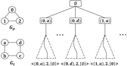
As shown in Figure 1, consider a pattern graph Gp = {0, 1, 2} and a target graph Gt = {a, b, c, d}. Suppose a worker exhaustively explores the branch starting with (0, a) and finds ms = 2. Then, the worker generates reuse information ⟨(0, a), 2, ∅⟩. Subsequently, the worker matches pattern vertex 0 with other target vertices, generating reuse information for each. Once all possibilities for vertex 0 are exhausted, vertex 0 is excluded. Later, when the branch starting with (1, a) is exhaustively searched, the worker generates reuse information ⟨(1, a), 2, {0}⟩. The set {0} indicates that there is no need to explore vertex 0 within the current branch.
4.2 Pruning Strategy
Our framework leverages shared information to determine whether the current search branch is worth exploring. We design pruning rules based on two types of shared information: the size of the current global best matching bsgo and the reuse information set RI. To implement this pruning strategy, each worker w maintains its own private variables, including the local best matching found so far M w lo , the set of excluded pattern vertices Bw in the current task, and the upper bound UBw of the current branch (computed using the adopted MCIS algorithm). The following introduces two pruning rules using the shared information.
Pruning Rule 1. If the upper bound of the current branch does not exceed the currently known best matching size (i.e., UBw ≤ max(|M w lo |, bsgo)), the search backtracks to the deepest unexplored node.
By definition of UBw , no matching obtained from the current branch can have size greater than UBw . Now consider the case where the pruning condition UBw ≤ max(|M w lo |, bsgo) holds. In this case, even in the most optimistic scenario (i.e., achieving the upper bound UBw ), the best possible matching obtainable from this branch is of size at most max(|M w lo |, bsgo), which is no larger than the size of the best matching already known. Hence, there is no benefit in further exploring this branch, and it can be safely pruned. The search then backtracks to the deepest unexplored node.
Pruning Rule 2. If the initial vertex pair of the current branch matches that of a reuse information ⟨(vi, uj), ms, S⟩ ∈ RI and satisfies either:
- S ⊂ Bw and ms ≤max(|M w lo |, bsgo) · Bw ⊆ S and ms + |S| - |Bw | ≤ max(|M w lo |, bsgo)
, then the search backtracks to the vertex vi.
Suppose the initial vertex pair of the current branch matches a reuse entry ⟨(vi, uj),ms, S⟩ ∈ RI. The pruning condition depends on the relation between Bw and S. In the first case, if S ⊂ Bw , then the current branch excludes at least all vertices that were excluded in the reuse information. Hence, its achievable matching size cannot exceed the recorded value ms. In the second case, if Bw ⊆ S, then the reuse information has a search space no larger than that associated with the current branch. Thus, in the most optimistic expansion, the best matching size attainable in this branch is ms + |S| - |Bw |. If the corresponding upper bound in either case does not exceed the currently known best matching size,
Algorithm 1: Prune
Input: The shared information bsgo and RI Output: The backtracking vertex v 1 v ←-1; 2 if satisfies Pruning Rule 1 then 3 v ← the deepest unexplored pattern vertex; 4 else if RI ̸= ∅ then 5 (vi, ui) ← initial vertex pair in the current branch; 6 if (vi, ui) satisfies Pruning Rule 2 then v ← vi ; 7 return v;then the branch cannot yield a better matching. Therefore, it is safely pruned, and the search backtracks to vertex vi.
4.3 Details of Pruning Procedure
The pruning strategy is implemented in Algorithm 1. The backtracking vertex v is initialized to -1 (Line 1). The algorithm first computes an upper bound following the adopted MCIS algorithm and checks whether pruning rule 1 is satisfied (Line 2). If so, the search backtracks to the deepest unexplored pattern vertex (Line 3). When the reuse information set RI is not empty, the algorithm obtains the initial vertex pair (vi, ui) of the current branch (Line 5). Then, it checks if this pair satisfies pruning rule 2. If satisfied, the algorithm should backtrack to the vertex vi (Line 6).
5 Our Parallel Framework
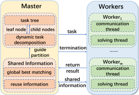
Our framework adopts a master-worker architecture , as illustrated in Figure 2.
Master: The master dynamically decomposes and assigns tasks to idle workers, while periodically collecting the size of the local best matchings and reuse information. It also broadcasts valuable shared information to all workers for effective pruning. Upon task completion or reaching the cutoff time, the master terminates all workers.
In Algorithm 2, the master initializes the global best matching size bsgo, the reuse information set RI, and the global best matching Mgo accordingly (Line 1). For each worker
Algorithm 2: Master
Input: Gp = (Vp, Ep), cutoff Output: the global best matchingMgo 1 bsgo ← 0, RI ←Mgo ← ∅; 2 idle[w] = 1 for each worker w; 3 while runtime < cutoff do 4 if ∃ worker w with idle[w] = 1 then 5 send a task with sets A and B to the worker w based on dynamic task decomposition; 6 idle[w] = 0; 7 if meet the requesting condition then 8 if ∃ worker w with idle[w] = 0 then 9 require |M w lo | and RI w new from worker w; 10 if |M w lo | > bsgo then bsgo ← |M w lo | ; 11 RI ← RI ∪ RI w new ; 12 broadcast bsgo and RI to workers; 13 if ∃ worker w with idle[w] = 0 and task is finished then 14 receive M w lo from worker w and idle[w] = 1; 15 if |M w lo | > |Mgo| then 16 Mgo ← M w lo and bsgo ← |M w lo |; 17 if finished all tasks then break ;18 send termination signal to the workers;
19 receive M w
20 returnMgo;
lo fromworkers and update Mgo;
w, we use idle[w] to indicate its status, where idle[w] = 1 means the worker is idle, and idle[w] = 0 means it is busy. Initially, all workers are set to idle, i.e., idle[w] = 1 for each worker (Line 2). Within the time limit, the master dynamically decomposes tasks and assigns them to idle workers, setting idle[w] = 0 for each worker (Lines 4-6). In Lines 7-9, the master periodically requests the local best matching size |M w lo | and newly generated reuse information RI w new from all workers (set to every 10 seconds). It then updates bsgo and RI (Lines 10-11), and broadcasts the latest bsgo and RI to all workers to achieve effective pruning (Line 12). When a worker completes its task, the master receives its local best matching M w lo and marks the worker as idle again (Line 14). If this M w lo outperforms the current global best matching, the master updates Mgo and bsgo accordingly (Lines 15-16). Once all tasks are completed or the cutoff time is reached, the master sends a termination signal to all workers (Line 18). Finally, the master receives all results and updates the global best matching Mgo based on these results (Line 19).
Worker: To improve computational and communication efficiency, each worker uses two threads: a communication thread for task reception, result reporting, and shared information exchange with the master, and a solving thread that runs the MCIS algorithm with the proposed pruning strategy.
Algorithm 3 describes the cooperation between the communication and the solving threads within a worker. The global variables in a worker include the local best matching Mlo, the newly generated reuse information set RInew, the reuse information set RI, the global best matching size
Algorithm 3: Worker
Input: Gp = (Vp, Ep), Gt = (Vt, Et) Output: the local best matchingMlo 1 Global Mlo ← RInew ← RI ← ∅, bsgo ← ms ← 0; 2 return Communication(); /* communication thread */ 3 Thread Communication(); 4 while do 5 if solving thread is idle then 6 receive a task with sets A and B from master; 7 Solving(A, B); 8 else if task is finished then sendMlo to master ; 9 else if meet the requesting condition then 10 send |Mlo| and RInew to master and RInew ← ∅; 11 receive bsgo and RI frommaster; 12 else if receive a termination signal then break ; 13 sendMlo to master; /* solving thread */ 14 Thread Solving(A,B); 15 Search(∅,A, Vp \ (A∪B),B, bsgo,RI);bsgo, and the maximum matching size ms under the current branch. First, these variables are initialized accordingly (Line 1). Then, the worker launches the communication thread (Line 2). When a task is received, the communication thread activates the solving thread to perform the computation.
As for the communication thread (Lines 3-13), it repeatedly performs the following operations: (1) When the solving thread is idle, it receives a new task from the master and wakes up the solving thread to start computation (Lines 5-7). (2) When the solving thread completes the task, it sends the local best matching Mlo to the master (Line 8). (3) When the master requests information (every 10 seconds), it sends the current best matching size |Mlo| and the newly reuse information RInew to the master, and receives the global best matching size bsgo and reuse information set RI from the master (Lines 9-11). (4) Upon receiving a termination signal, it exits the loop (Line 12). Within the loop, if no communication is required, the communication thread sleeps for 1 second to avoid invalid queries. Finally, it sends the local best matching Mlo to the master (Line 13).
As for the solving thread, it invokes the Search function to perform the solving process (Line 15). The Search function is described in Algorithm 4. The six input parameters include: the current matching Mc (initialized as empty), the priority matching pattern vertex set A, the remaining pattern vertex set Vr (initialized as Vp\(A∪B)), the excluded pattern vertex sets S ( initialized as the current task's set B), as well as the globally shared information bsgo and RI.
If the current matching Mc has a larger size than Mlo and exceeds the value of ms, then Mlo and ms are updated (Lines 1-2). The algorithm then determines whether to continue the search based on the shared information bsgo and RI from the
Algorithm 4: Search
Input: Mc, A, Vr , S, bsgo, RI Output: The backtracking vertex v′ 1 if |Mc| > |Mlo| then Mlo ←Mc ; 2 if |Mc| >ms then ms ← |Mc| ; 3 v′ ←Prune(bsgo,RI); 4 if v′ ̸= -1 then return v′ ; 5 if A ̸= ∅ then vi ← pop(A) ; 6 else vi ← select a pattern vertex from Vr ; 7 for each uj ∈ Vt can be matched to vi do 8 Mc ←Mc ∪ {(vi, uj)}; 9 v′ ← Search(Mc, A, Vr, S, bsgo, RI); 10 Mc ←Mc \ {(vi, uj)}; 11 if v′ ̸= -1 and v′ ̸= vi then return v′ ; 12 if |Mc| == 0 and |S| < thrd then 13 RInew ← RInew ∪ {⟨(vi, uj ), ms, S⟩} and ms ← 0; 14 Vr ← Vr \ {vi} and S ←S ∪ {vi}; 15 v′ ←Search(Mc,A, Vr, S, bsgo,RI); 16 return v′ ;master (Line 3). If the returned vertex is not -1, the search backtracks to vertex v′ (Line 4). Next, the algorithm prioritizes obtaining a vertex from the set A (Line 5). The algorithm selects the last vertex from the set A each time. If A is empty, it selects a vertex vi from Vr based on the adopted MCIS algorithm (Line 6). For the vertex vi, the algorithm traverses all vertices uj in the target graph that can be matched with vi according to the adopted MCIS algorithm, and recursively invokes itself to extend the matching (Line 9). If pruning occurs during the search process, the search backtracks to vertex v′ (Line 11). When the search of a branch is completed, a piece of reuse information is generated and stored in RInew (Line 13). As reuse information with a large set S has low utility and can only prune a relatively limited search space, we only collect reuse information where |S| < thrd. In our experiments, thrd is set to 10. Subsequently, the algorithm explores the search space that does not include vertex vi, moves vi from the remaining vertex set Vr to the set S, and continues the recursive search (Lines 14-15).
6 Experimental Evaluation
In this section, we apply our framework to enhance the stateof-the-art MCIS algorithm and evaluate the performance of the proposed algorithm across a broad range of benchmarks.
6.1 Experiment Preliminaries
We adopt 8 benchmarks 1 with 15,396 instances in total, following previous works [Liu et al., 2020; Liu et al., 2023; Wang et al., 2024; Kothalawala et al., 2025; Yu et al., 2025]. (1) images-CVIU11 [Damiand et al., 2011] has 6,278 segmented image instances, with 43 pattern graphs (22-151 vertices) and 146 target graphs (1,072-5,972 vertices). (2) meshes-CVIU11 [Damiand et al., 2011] has 3,018 instances from meshes modeling 3D objects, with 6 pattern graphs (40-199 vertices) and 503 target graphs (208-5,873 vertices). (3) images-PR15 [Solnon et al., 2015] has 24 segmented image instances, with 24 pattern graphs (4-170 vertices) and 1 target graph (4,838 vertices). (4) scalefree [Solnon, 2010] includes 100 random instances, where target graphs have 200-1,000 vertices and pattern graphs comprise 90% of the target vertices. (5) si [Solnon, 2010] has 1,170 instances, with target graphs (200-1,296 vertices) and pattern graphs (20%-60% of target vertices). (6) phase [McCreesh et al., 2017] comprises 200 instances selected close to the satisfiable-unsatisfiable phase transition, with a pattern graph with 30 vertices and a target graph with 150 vertices. (7) LV [Solnon, 2010] has 1,176 instances, using 49 graphs (10-128 vertices) as both pattern and target graphs. (8) LargerLV extends LV with 3,430 instances, using the same 49 pattern graphs and 70 new target graphs (138-6,671 vertices).
1 http://liris.cnrs.fr/csolnon/SIP.html
We evaluated the proposed algorithm against sequential and parallel algorithms. For sequential algorithms, we select four state-of-the-art McSplit variants: McSplitDAL [Liu et al., 2023], McSplitDSB [Kothalawala et al., 2025], RRSplit [Yu et al., 2025], and McSplitDALPR [Calabrese et al., 2026]. For parallel algorithms, we adopted a CPU-based multi-threaded parallel algorithm v2 [Quer et al., 2020] and a parallel version of the McSplit algorithm [Hoffmann et al., 2018], which we denote as ParaMcSplit in this paper. To enhance the comparison, we integrate the four sequential algorithms into a portfolio named PortfolioMCIS. Specifically, for each instance, PortfolioMCIS runs the four algorithms in parallel, and its performance is the optimal matching obtained by the first algorithm that completes within the time limit.
Since RRSplit performs best among the sequential algorithms, we extended it into a parallel version using our framework, denoted as ParaRRS 2 . Our algorithm is parallelized with OpenMPI. ParaRRS and all compared algorithms are implemented in C or C++ and compiled with g++ using the -O3 optimization flag. All experiments are conducted on the servers equipped with an Intel Xeon Gold 6238 CPU (2.10 GHz) and 512 GB of RAM, running Ubuntu 22.04. For each instance, the time limit of all algorithms is 1800 seconds. In the comparative experiments, PortfolioMCIS requires at least 4 threads to run its four constituent algorithms in parallel. Therefore, we configured PortfolioMCIS, ParaMcSplit and v2 to use 4 threads. Since v2 runs with 8 threads in their work, we also include this version in our experimental evaluation. Accordingly, our ParaRRS algorithm was set to use 4 processes (one master and three workers).
6.2 Comparative Experiment
To clearly show the overall performance of ParaRRS and its competitors, we followed previous studies [Liu et al., 2020; Liu et al., 2023] by excluding two types of instances: (1) 976 easy instances solved by all algorithms within 10 seconds; (2) 12,222 extremely hard instances unsolvable by any algorithm within the time limit. There are 2,198 remaining instances.
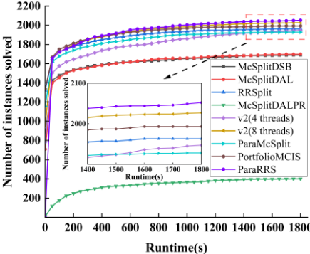
According to the time taken by each algorithm to find the optimal matching, we illustrate the number of solved instances for all algorithms in Figure 3. ParaRRS solves 2,052 instances, outperforming all competitors. Notably, ParaRRS can solve 52 instances unsolved by all competitors. When compared with the parallel algorithms PortfolioMCIS, v2(4 threads), v2(8 threads), and ParaMcSplit, ParaRRS solved 59, 105, 25, and 124 more instances, corresponding to performance improvements of 3.0%, 5.4%, 1.2%, and 6.4%, respectively. When compared with the sequential algorithms, ParaRRS achieves superior performance, solving 89, 362, 354, and 1,651 more instances than RRSplit, McSplitDSB, McSplitDAL, and McSplitDALPR, respectively. The results show that ParaRRS exhibits superior solving ability compared to both parallel and sequential algorithms. In particular, the solving performance of ParaRRS improves upon RRSplit by 4.5%, demonstrating that the parallelization strategies of our framework effectively speed up the search process.
2 https://github.com/yiyuanwang1988/Parallel-MCSP.git
6.3 Scalability Analysis
To evaluate the scalability and generality of our framework, we parallelize three state-of-the-art sequential MCIS algorithms, RRSplit, McSplitDAL and McSplitDSB, which are denoted as ParaRRS, ParaDAL and ParaDSB, respectively. To further assess their scalability, we randomly select one extremely hard unsolved instance from each benchmark in the comparative experiment. The images-PR15 benchmark is excluded, as all its instances can be solved within the time limit by the three sequential algorithms. We then tested these parallel algorithms on the selected instances using 4 to 64 processes. The experimental results are presented in Table 1. In the table, result denotes the size of the found best matching, and time denotes the time to find it. Results for instances solved to optimality are marked in bold.
The results clearly show that all algorithms exhibit a significant performance improvement as the number of processes increases. Specifically, with more processes, these three parallel algorithms find larger matchings or achieve the same matching size in less time. Notably, these three parallel algorithms solved the hard instances pattern10 target27
| Instance | Algorithms | np=4 | np=8 | np=16 | np=32 | np=64 | |||||
|---|---|---|---|---|---|---|---|---|---|---|---|
| result | time | result | time | result | time | result | time | result | time | ||
| ParaDAL | 123 | 201.4 | 123 | 198.3 | 123 | 69.6 | 123 | 58.0 | 123 | 48.4 | |
| pattern10 target27 | ParaDSB | 100 | 39.1 | 107 | 1691.2 | 123 | 1049.6 | 123 | 266.8 | 123 | 145.4 |
| ParaRRS | 106 | 1282.7 | 123 | 313.6 | 123 | 218.7 | 123 | 78.7 | 123 | 57.7 | |
| ParaDAL | 101 | 1643.6 | 101 | 94.0 | 101 | 75.0 | 120 | 34.2 | 120 | 1.9 | |
| g38 g76 | ParaDSB | 99 | 443.0 | 99 | 11.0 | 99 | 11.0 | 120 | 33.3 | 120 | 23.2 |
| ParaRRS | 107 | 1086.0 | 121 | 665.6 | 121 | 299.8 | 121 | 0.0 | 121 | 0.0 | |
| ParaDAL | 64 | 124.2 | 64 | 33.5 | 64 | 21.6 | 64 | 15.2 | 66 | 1687.7 | |
| g42 g43 | ParaDSB | 64 | 45.9 | 64 | 16.0 | 64 | 16.0 | 64 | 16.1 | 64 | 15.1 |
| ParaRRS | 64 | 5.5 | 66 | 1458.0 | 66 | 1444.0 | 67 | 251.5 | 67 | 74.1 | |
| ParaDAL | 159 | 355.1 | 159 | 3.8 | 161 | 65.7 | 161 | 0.0 | 161 | 0.0 | |
| pattern3 target56 | ParaDSB | 159 | 1224.3 | 159 | 0.5 | 161 | 174.1 | 161 | 0.0 | 161 | 0.0 |
| ParaRRS | 159 | 577.3 | 159 | 11.3 | 161 | 49.4 | 161 | 6.0 | 161 | 4.9 | |
| ParaDAL | 23 | 84.0 | 23 | 65.3 | 23 | 50.9 | 23 | 50.7 | 23 | 40.8 | |
| phase-30-150-0.84-0.76-0.76-7 | ParaDSB | 23 | 110.0 | 23 | 87.0 | 23 | 51.6 | 23 | 52.4 | 23 | 43.4 |
| ParaRRS | 23 | 110.3 | 23 | 86.6 | 23 | 51.4 | 23 | 51.7 | 23 | 42.0 | |
| ParaDAL | 94 | 1415.8 | 95 | 788.2 | 132 | 0.0 | 132 | 0.0 | 139 | 1335.0 | |
| A.15 | ParaDSB | 94 | 858.4 | 96 | 1422.4 | 132 | 1.0 | 132 | 0.0 | 139 | 785.6 |
| ParaRRS | 94 | 785.5 | 96 | 1268.3 | 132 | 0.0 | 132 | 0.0 | 139 | 705.1 | |
| ParaDAL | 429 | 1660.5 | 429 | 1655.9 | 434 | 505.8 | 518 | 1174.9 | 518 | 184.1 | |
| si4 m4D m1296.00 | ParaDSB | 429 | 1189.3 | 429 | 1183.0 | 434 | 1005.4 | 518 | 678.3 | 518 | 87.1 |
| ParaRRS | 434 | 1287.8 | 434 | 1235.6 | 434 | 569.5 | 518 | 414.0 | 518 | 53.4 | |
and si4 m4D m1296.00 with 16 and 32 processes, respectively. Furthermore, ParaRRS solved g38 g76 using just 8 processes. For hard phase instances, although all algorithms achieve the same matching size under different process counts, their runtime with 64 processes is only half that with 4 processes. This demonstrates that our framework is not limited to improving a single algorithm, it enhances the number of solvable instances and the overall solving efficiency across all three algorithms. These findings strongly validate the outstanding scalability and generality of our framework.
6.4 Ablation Study
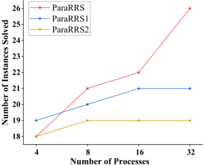
To verify the effectiveness of the proposed strategies, we compare ParaRRS with two variants:(1) ParaRRS1 does not employ dynamic task decomposition method. Instead, the master adopts the same task decomposition approach as in [Quer et al., 2020], where each node in the task tree corresponds to a partial matching and the remaining unmatched vertices. (2) ParaRRS2 removes our pruning strategy, and each worker only prunes using its local best matching.
We sampled 10 instances from each benchmark, resulting in a total of 80 instances. Figure 4 shows the number of instances successfully solved by ParaRRS and its two variants. As the number of processes increases, ParaRRS solves more instances than both variants. Notably, with 32 processes, it solves 26 instances, achieving a performance gain of 23.8% over ParaRRS1 and 36.8% over ParaRRS2. The dynamic task decomposition strategy adopted by ParaRRS relies on vertex scoring information collected during the search process to guide partitioning. This mechanism struggles to fully leverage its advantages when the number of processes is small, and thus it finds one fewer optimal matching than ParaRRS1 when running with 4 processes. Although ParaRRS exhibits comparable performance to both variants when using 4 processes, its dynamic task decomposition method enables more efficient utilization of parallel computational resources as the number of processes increases. Simultaneously, the proposed pruning strategy can generate more useful shared information, thereby significantly improving the search efficiency.
7 Conclusion
This paper proposes a parallel framework for solving the MCIS. The framework adopts a master-worker architecture that integrates a dynamic task decomposition method and a novel pruning strategy. Experimental results show that the algorithm enhanced by our framework outperforms both stateof-the-art sequential and existing parallel algorithms.
Acknowledgments
This work is supported by National Cryptologic Science Fund of China 2025NCSF02046, NSFC under Grant No. 61806050.
@inproceedings{ijcai2026p709,
  title     = {A Parallel Framework for the Maximum Common Induced Subgraph Problem},
  author    = {Wu, Jieyu and Zhang, Quan and Wang, Yiyuan and Pan, Shiwei and Gao, Jian},
  booktitle = {Proceedings of the Thirty-Fifth International Joint Conference on
               Artificial Intelligence, {IJCAI-26}},
  publisher = {International Joint Conferences on Artificial Intelligence Organization},
  editor    = {Diego Calvanese},
  pages     = {6370--6378},
  year      = {2026},
  month     = {8},
  note      = {Main Track},
  doi       = {10.24963/ijcai.2026/709},
  url       = {https://doi.org/10.24963/ijcai.2026/709},
}
TY - CPAPER TI - A Parallel Framework for the Maximum Common Induced Subgraph Problem AU - Wu, Jieyu AU - Zhang, Quan AU - Wang, Yiyuan AU - Pan, Shiwei AU - Gao, Jian T2 - Proceedings of the Thirty-Fifth International Joint Conference on Artificial Intelligence, IJCAI-26 PB - International Joint Conferences on Artificial Intelligence Organization PY - 2026 SP - 6370 EP - 6378 DO - 10.24963/ijcai.2026/709 UR - https://doi.org/10.24963/ijcai.2026/709 ER -Copied
Machine-readable versions of this paper, for tools and AI agents:





