
FastLCD: Fast Label Coordinate Descent for the Efficient Optimization of 2D Label MRFs
Proceedings of the Twenty-Fifth International Joint Conference on Artificial Intelligence. Pages 624-629.
Abstract
Recently, MRFs with two-dimensional (2D) labels have proved useful to many applications, such as image matching and optical flow estimation. Due to the huge 2D label set in these problems, existing optimization algorithms tend to be slow for the inference of 2D label MRFs, and this greatly limits the practical use of 2D label MRFs. To solve the problem, this paper presents an efficient algorithm, named FastLCD. Unlike previous popular move-making algorithms (e.g., α-expansion) that visit all the labels exhaustively in each step, FastLCD optimizes the 2D label MRFs by performing label coordinate descents alternately in horizontal, vertical and diagonal directions, and by this way, it does not need to visit all the labels exhaustively. FastLCD greatly reduces the search space of the label set and benefits from a lower time complexity. Experimental results show that FastLCD is much faster, while it still yields high quality results.
- [Baker et al., 2011] Simon Baker, Daniel Scharstein, JP Lewis, Stefan Roth, Michael J Black, and Richard Szeliski. A database and evaluation methodology for optical flow. IJCV, 92(1), 2011.
- [Besag, 1986] Julian Besag. On the statistical analysis of dirty pictures. Journal of the Royal Statistical Society, 48(3), 1986.
- [Boykov et al., 2001] Yuri Boykov, Olga Veksler, and Ramin Zabih. Fast approximate energy minimization via graph cuts. TPAMI, 23(11), 2001. Duchenne et al., 2011] Olivier Duchenne, Armand Joulin, and Jean Ponce. A graph-matching kernel for object cate- gorization. In ICCV, 2011.
- [Friedman et al., 2010] Jerome Friedman, Trevor Hastie, and Rob Tibshirani. Regularization paths for generalized lin- ear models via coordinate descent. Journal of statistical software, 33(1):1, 2010.
- [Glocker et al., 2008] Ben Glocker, Nikos Paragios, Nikos Komodakis, Georgios Tziritas, and Nassir Navab. Optical flow estimation with uncertainties through dynamic mrfs. In CVPR, 2008.
- [Ishikawa, 2003] Hiroshi Ishikawa. Exact optimization for markov random fields with convex priors. TPAMI, 25(10), 2003.
- [Kolmogorov and Zabin, 2004] Vladimir Kolmogorov and Ramin Zabin. What energy functions can be minimized via graph cuts? TPAMI, 26(2), 2004.
- [Kolmogorov, 2006] Vladimir Kolmogorov. Convergent tree- reweighted message passing for energy minimization. TPAMI, 28(10), 2006.
- [Kumar and Torr, 2008] M Pawan Kumar and Philip HS Torr. Improved moves for truncated convex models. In NIPS, 2008. [Ladicky et al., 2010]
- Lubor Ladicky, Paul Sturgess, Chris Russell, Sunando Sengupta, Yalin Bastanlar, William Clocksin, and Philip Torr. Joint optimisation for object class segmentation and dense stereo reconstruction. 2010.
- [Ladicky et al., 2012] Lubor Ladicky, Philip Torr, and An- drew Zisserman. Latent svms for human detection with a locally affine deformation field. In BMVC, 2012.
- [Lempitsky et al., 2007] Victor Lempitsky, Carsten Rother, and Andrew Blake. Logcut-efficient graph cut optimization for markov random fields. In ICCV, 2007.
- [Lempitsky et al., 2008] Victor Lempitsky, Stefan Roth, and Carsten Rother. Fusionflow: Discrete-continuous optimiza- tion for optical flow estimation. In CVPR, 2008.
- [Ling and Jacobs, 2005] Haibin Ling and David W. Jacobs. Deformation invariant image matching. In ICCV, 2005.
- [Liu et al., 2014] Kangwei Liu, Junge Zhang, Kaiqi Huang, and Tieniu Tan. Deformable object matching via deforma- tion decomposition based 2d label mrf. In CVPR, 2014.
- [Liu et al., 2015] Kangwei Liu, Junge Zhang, Peipei Yang, and Kaiqi Huang. Grsa: Generalized range swap algorithm for the efficient optimization of mrfs. In CVPR, 2015.
- [Pedersoli et al., 2014] Marco Pedersoli, Radu Timofte, Tinne Tuytelaars, and Luc Van Gool. Using a deforma- tion field model for localizing faces and facial points under weak supervision. In CVPR, 2014.
- [Schlesinger and Flach, 2006] Dmitrij Schlesinger and Boris Flach. Transforming an arbitrary minsum problem into a binary one. TU, Fak. Informatik, 2006.
- [Shabou et al., 2009] Aymen Shabou, Florence Tupin, and Jérôme Darbon. A graph-cut based algorithm for approxi- mate mrf optimization. In ICIP, 2009.
- [Shekhovtsov et al., 2007] Alexander Shekhovtsov, Ivan Kovtun, and Vaclav Hlavac. Efficient mrf deformation model for non-rigid image matching. In CVPR, 2007.
- [Szeliski et al., 2008] Richard Szeliski, Ramin Zabih, Daniel Scharstein, Olga Veksler, Vladimir Kolmogorov, Aseem Agarwala, Marshall Tappen, and Carsten Rother. A com- parative study of energy minimization methods for mrfs with smoothness-based priors. TPAMI, 30(6), 2008.
- [Tappen and Freeman, 2003] Marshall F Tappen and William T Freeman. Comparison of graph cuts with belief propagation for stereo using identical mrf parameters. In ICCV, 2003.
References were extracted automatically from the PDF and may contain errors.
Full text extracted automatically from the PDF; figures, tables and equations may differ. The PDF is the version of record.
1 Introduction
Markov random fields have become an important tool for many problems in computer vision and machine learning areas. Recently, two-dimensional (2D) label MRFs have attracted more and more attention in many AI tasks, such as image matching [Shekhovtsov et al., 2007; Liu et al., 2014], optical flow estimation [Lempitsky et al., 2008], object classification [Duchenne et al., 2011], detection [Pedersoli et al., 2014; Ladicky et al., 2012] and jointly segmentation and stereo matching [Ladicky et al., 2010]. These tasks refer to assigning a two-dimensional label (xp↪ yp) to every pixel p 2 P. For example, the labels xp and yp in image matching represent the displacements of pixels in horizontal and vertical directions, respectively. In jointly segmentation and stereo matching, xp and yp denote the categories of objects and the disparities of pixels, respectively.
In the last decades, many successful algorithms have been proposed for the optimization of MRFs, such as ↵- expansion [Boykov et al., 2001; Kolmogorov and Zabin, 2004], sequential belief propagation (BPS) [Tappen and Freeman, 2003], and sequential tree-reweighted message passing
(TRWS) [Kolmogorov, 2006]. State-of-the-art optimization algorithms usually exhibit good optimality properties and yield high-quality solutions on the MRF models. In fact, the accuracy of the best known algorithms sometimes exceeds the demand of the applications by a wide margin [Szeliski et al., 2008]. However, these algorithms tend to be slow, and the run time of most existing algorithms increase rapidly as the size of the label set increases. For example, the run time taken by ↵-expansion grows linearly with the increase of label size [Lempitsky et al., 2007], because it needs to consider all the labels exhaustively in the iterative optimization. Unfortunately, the label space is usually huge in the applications of 2D label MRFs. For example, [Lempitsky et al., 2008] formulates the problem of optical flow estimation as solving an MRF with 2D discrete labels. There are about 1000 labels in the problem. It takes about an hour to process one single frame pair, although state-of-the-art accuracy is obtained from this algorithm. To optimize the 2D label MRFs efficiently, [Duchenne et al., 2011] develops the curve expansion algorithm. However, the applicability of curve expansion is limited because of two major problems: (i) it is limited in the type of energies it can handle (only convex energy functions); (ii) it still takes a lot of time in the optimization because a huge graph is required to compute a labeling in each iteration.
Therefore, it is a challenging problem to develop an efficient algorithm that has a lower time complexity of label size, while ensuring it is applicable to a large range of energy functions. To solve this problem, this paper presents an efficient algorithm named fast label coordinate descent (FastLCD).Unlike previous move-making algorithms (e.g., ↵-expansion [Boykov et al., 2001]) that consider the labels exhaustively, FastLCD utilizes the fact that the label set is two-dimensional, and restricts the pixels to change their labels along horizontal, vertical and diagonal directions in the 2D label space. We call the labeling updating along the fixed direction as a label coordinate descent (LCD). By performing the LCD, FastLCD does not need to visit all the labels exhaustively and greatly reduces the search space in the iterative optimization. FastLCD benefits from a lower complexity of O(m+n) in each iteration, where m and n are the size of the 2D label set.
The FastLCD executes the label coordinate descent in each direction by a series of moves. For example, in a horizontal move, every pixel is allowed to change their horizontal labels to a new one, while keeping their vertical label unchanged. In each move, FastLCD only needs to construct a binary graph instead of a huge graph as in curve expansion. We construct the binary graph using the graph cuts techniques developed in [Kolmogorov and Zabin, 2004]. However, this method requires the submodular condition, which is hard to be satisfied in many popular energy functions. To allow FastLCD to handle more general functions, we propose an approximate graph construction for the cases where the submodular condition is not satisfied. We also provide a theoretical guarantee for this approximate construction, and show that it holds an upper bound of the obtained energy. Unlike ↵-expansion which is only applicable to metric 1 energy functions or curve expansion that is limited to only convex energy functions, the approximate graph construction allows FastLCD to handle arbitrary semimetric energy functions.
The idea of our FastLCD is similar to coordinate descent [Friedman et al., 2010] for convex optimization, which performs line search along one coordinate direction. The difference is that FastLCD does line search in a discrete label space instead of a continuous space, while the line search is executed by a series of moves rather than gradient descent.
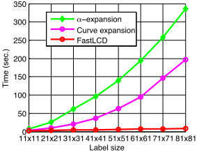
We evaluate FastLCD on both synthetic data and vision problems of image matching and optical flow estimation. Experiments show that FastLCD offers a great speedup over related methods (e.g., it is 40 times faster than ↵-expansion and 22 times faster than curve expansion when the label space is 81⇥81 as shown in Fig. 1), while still yields competitive solutions. We will publish the code for academic application.
2 2D label MRF optimization
Preliminaries An MRF is defined over an undirected graph G =(P↪ E), where P is the set of pixels, and E is the set of edges connecting neighboring pixels. The task of MRFs is to assign every pixel p a label fp 2 L. The goal of optimizing the MRFs is to obtain the labeling f that minimizes the following energy:
1 Here, metric means that the pairwise function should satisfy (i) ✓(↵↪ β) = 0 , ↵ = β; (ii) ✓(↵↪ β) = ✓(β↪ ↵) ≥ 0 and (iii) ✓(↵↪ β) ✓(↵↪ γ) + ✓(γ↪ β). If the pairwise function satisfies only (i) and (ii), it is called semimetric.
where ✓p and ✓pq denote the unary and pairwise potentials respectively. Typically, if the label set L is one-dimensional, we have
Theorem 1 ( [Schlesinger and Flach, 2006]). The minimum of energy function E(f) can be exactly obtained via graph cuts, if and only if ✓pq(fp↪ fq) satisfies the submodular condition
for any pair of labels i,j 2 L.
The task of 2D label MRFs is to assign every pixel p a two-dimensional label fp = (xp↪ yp), and the label set is a two-dimensional label space L=X⇥Y. Unfortunately, the submodular condition is seldom satisfied in the energies of the 2D label MRFs. These algorithms (e.g., [Ishikawa, 2003; Shabou et al., 2009; Liu et al., 2015]) which are popular but restricted to the case of one-dimensional labels cannot be used for the optimization of 2D label MRFs.
Label coordinate descent To make the optimization of 2D label MRFs easier, we consider a direction #, and restrict the labeling f to be updated along the fixed direction # in the label space. By this way, the optimization of 2D label MRFs is naturally transformed to the one-dimensional case:
where f # p 2 L#p , and L#p denotes the label set along the fixed direction # at the current assignment fp.
We call the minimization of E(f # ) in (3) as a label coordinate descent (LCD). Assume we start with an initial labeling f (0) , and get a sequence of labeling f (1) ↪ · · · ↪ f (n) by performing a series of LCD. Since each LCD minimizes the energy E(f # ), we have
Thus, a local minimum will be reached when there is no descent can be found to decrease E(f). By this way, the optimization of a 2D label MRF could be solved by a series of subproblem over one-dimensional label case.
Let g(u↪ v) = ✓(fp↪ fq) denote the pairwise function, where u = ♣xp - xq♣ and v = ♣yp - yq♣.
Theorem 2. If the pairwise function g(u↪ v) is a convex function, then E(f # ) satisfies the submodular condition in Theorem 1. In other word, E(f # ) in (3) can be exactly optimized via graph cuts 2 .
Theorem 1 specifies the cases when the label coordinate descent over all directions # can be exactly solved by via graph cuts [Ishikawa, 2003]. However, it still requires a huge graph needs to be constructed in the graph cuts method of [Ishikawa, 2003], while it takes a lot of time to perform all the possible label coordinate descents. As the efficiency is vitally important to real problems, this forces the development of efficient approximate algorithms.
2 Due to the limit of the space, we have to omit the proof here. We would like to public it in the supplementary materials in the future.
3 The FastLCD
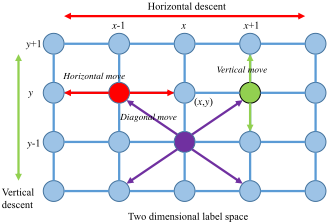
In this section, we present the FastLCD algorithm, which efficiently optimizes 2D label MRFs by iteratively performing label coordinate descent in horizontal, vertical and diagonal lines instead of all directions (see Fig. 2).
In the FastLCD, every label coordinate descent decreases E(f) by making a series of moves, each of which provides the pixels a choice of two labels. For example, one horizontal move considers a label ↵ 2 X, and it allows every pixel p 2 P (assume its current label is (xp↪ yp)) to change its horizontal label xp to ↵, while keeping its vertical label yp unchanged. Within this move, the energy E(f) can be effectively decreased by finding a better labeling.
We initialize FastLCD by minimizing ✓p(fp), which can be solved extremely fast. Each move updates the labeling f if it yields a lower energy E(f 0 ) <E(f). The FastLCD reaches a local minimum and converges when no move can be found to decrease E(f). The FastLCD algorithm is shown in Algorithm 1, and we call the steps 2-5 a cycle of iterations. In each cycle, the horizontal descent performs m horizontal moves, while the vertical descent needs n vertical moves. Therefore, FastLCD has a lower time complexity of O(m+n) in each cycle instead of O(m · n) as in previous move-making algorithm, e.g., ↵-expansion.
3.1 Horizontal and vertical moves
The label coordinate descents in horizontal and vertical directions optimize E(f) by performing a series of horizontal and vertical moves, respectively. We explain only the horizontal moves for brevity, and similar arguments apply to the vertical moves.
In the FastLCD, each horizontal move considers a horizontal label ↵ 2 X, and allows every pixel p 2 P to retain its current label (xp↪ yp) or change (xp↪ yp) to (↵↪ yp). Let f ↵h p represent (↵↪ yp), where the superscript ↵h denote the horizontal component of f ↵h p is ↵. Each horizontal move minimizes the following energy
where f h p 2 ¶fp↪ f ↵h p ♦, and the energy E(f h ) has the following property:
Algorithm 1 The FastLCD Algorithm
Initialization:
1: Initialize the labeling f.
Iteration:
- 2: repeat
- 3: Perform the horizontal moves for each label ↵ 2 X: i. Find f 0 = argminE(f h ) by st-mincut, where f h p 2 ¶(xp↪ yp)↪ (↵↪ yp)♦; ii. If E(f 0 ) < E(f), set f := f 0 .
- 4: Perform the vertical moves for each label β 2 Y: i. Find f 0 = argminE(f v ) by st-mincut, where f v p 2 ¶(xp↪ yp)↪ (xp↪ β)♦;
- If E(f 0 ) < E(f), set f := f 0 .
- 5: Perform diagonal moves for each pair of labels (↵, β) 2 ¶(1↪ 1)↪ (1↪ -1)↪ (-1↪ 1)↪ (-1↪ -1)♦: i. Find f 0 = argminE(f d ) by st-mincut, where f d p 2 ¶(xp↪ yp)↪ (xp + ↵↪ yp + β)♦; ii. If E(f 0 ) < E(f), set f := f 0 .
- 6: until No moves can be found to decrease E(f). Output:
- 7: Return the labeling f.
Theorem 3. If the pairwise function ✓(fp↪ fq) can be represented as ✓(fp↪ fq) = ✓1(xp↪ xq) + ✓2(yp↪ yq) (i.e. g(u↪ v) = g1(u) + g2(v)), and ✓1(xp↪ xq), ✓2(yp↪ yq) are metric, then each term ✓(f h p ↪ f h q ) satisfies the submodular condition, i.e., E(f h ) in (4) can be exactly minimized via graph cuts.
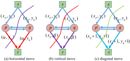
Theorem 3 specifies the cases when the energy E(f h ) in (4) can be exactly minimized via graph cuts (Fig. 3(a)).
Approximate move Unfortunately, many energy functions which have been widely used in 2D label MRFs do not satisfy the conditions in Theorem 3. To allow FastLCD to handle more general energy functions, we provide an effective method to approximate the optimal move.
Let (p↪ q) 2 ˆ E denote the sets of edges whose pairwise term ✓pq (f h p ↪ f h q ) that does not satisfy the submodular condition.
We rewrite the pairwise potentials for (p↪ q) 2 ˆ E:
The submodular condition of Eq. (2) is satisfied by setting:
Then, we have ˆapq + ˆbpq = ˆ cpq + ˆ dpq. The new energy in the follows can be exactly solved via graph cuts:
where ˆ ✓pq (f h p ↪ f h q ) is defined by Eq. (6), if (p↪ q) 2 ˆ E; otherwise, ˆ ✓pq (f h p ↪ f h q ) = ✓pq(f h p ↪ f h q ).
Let λpq = ∆pq tpq , where 0 λpq 1, we have the following guarantee
Theorem 4. Let f ⇤ be a global optimum of E(f h ), and ˆ f be a global minimum of ˆE(f h ). Then, we have E( ˆ f ) γE(f ⇤ ), where
Proof. With equations in (6), we obtain
Adding the unary potential to both sides of the inequality above, we obtain (1 - λmax)E( ˆ f) ˆE( ˆ f ),
Since ˆ f is the global minimum of ˆE(f h ), we have ˆE( ˆ f) ˆE(f ⇤ ), and thus, (1-λmax)E( ˆ f ) (1 + λmax)E(f ⇤ ).
3.2 Diagonal moves
The diagonal descent updates the labeling f along the diagonal directions by a series of diagonal moves, each of which considers a gradient from ¶(1↪ 1)↪ (1↪ -1)↪ (-1↪ 1)↪ (-1↪ -1)♦. Without loss of generality, we explain the diagonal move with the gradient of (1↪ 1), and similar arguments apply to other cases. The diagonal move on gradient (1↪ 1) allows every pixel p 2 P to either retain its current label (xp↪ yp) or change (xp↪ yp) to (xp+1↪ yp+1).
Let fp denote (xp↪ yp), and f p denote (xp+1↪ yp+1). The diagonal move minimizes the following energy:
where f d p 2 ¶fp↪ f p ♦.
Theorem 5. Assuming g(u↪ v) = ✓(fp↪ fq), if g(u↪ v) is a convex function, then each term ✓(f d p ↪ f d q ) satisfies the submodular condition, where f d p 2 ¶fp↪ f p ♦. In other words, E(f d ) in (9) can be exactly minimized via graph cuts.
Proof. Because g(u↪ v) is convex, we have
Let x1 = ♣xp-xq-1♣+♣xp-xq+1♣ 2 and y1 = ♣yp-yq-1♣+♣yp-yq+1♣ 2 . We have ♣xp-xq♣x1, and ♣yp-yq♣y1. Using Eq. (10), we obtain
Thus, ✓(fp↪ fq)+✓(f p ↪ f q ) ✓(fp↪ f q )+✓(f p ↪ fq) is satisfied for any term ✓(f d p ↪ f d q ).
Theorem 5 implies that if g(u↪ v) is a convex function, the diagonal moves can be exactly solved via graph cuts (Fig. 3(c)). If the pairwise term ✓(f d p ↪ f d q ) does not satisfy submodular condition, the diagonal move can be approximately solved by the method described in Sec. 3.1.
4 Experiments
In this section, we test the FastLCD algorithm on both synthetic data and real vision problems of image matching and optical flow estimation. We evaluate FastLCD on several different energy functions to verify its effectiveness on different types of energy functions. In the implementation of ↵-expansion, we use the approximate graph construction proposed in Sec. 3.1 to allow it to handle arbitrary semimetric energy functions.
4.1 Data and parameter setting
Image matching Given two images, the objective of image matching is to get the feature correspondence between the two images. To solve this problem, the first image (image1) is distorted to match the second one (image2). This can be naturally formulated as optimizing a 2D label MRFs [Shekhovtsov et al., 2007], where P denotes the set of pixels in image1 and the label (x↪ y) represents the 2D displacements of pixels.
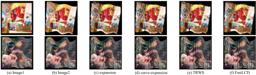
In this experiment, we use two image pairs chosen from the dataset of [Ling and Jacobs, 2005], and the image are shown in Fig. 5. The size of label space is set as 25 ⇥ 25. For the pairwise term, we choose g(u↪ v)=k(u2 +v2 ), and set k = 1.
200%
100%
1s
10s
100s
1,000s
(a) Pair1: energy vs. time
0s
0
ICM Expansion Swap BPS TRWS FastLCD curve-expan
(b) Pair1: time of per cycle vs. cycle numbers
1s
100s
1000s
(c) Pair2: energy vs. time
10
0
ICM Expansion Swap BPS TRWS FastLCD curve-expan
(d) Pair2: time of per cycle vs. cycle numbers
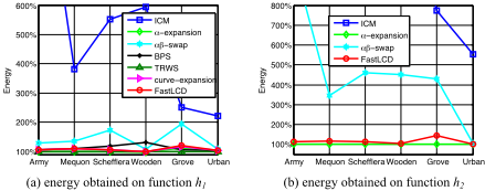
Optical flow The task of optical flow estimation is to obtain a two-dimensional flow vector at each pixel. In this problem, the continuous flows are represented by 2D discrete labels [Glocker et al., 2008]. In the experiment, we use the images fromMiddlebury dataset [Baker et al., 2011], which is a public benchmark for optical flow estimation.
We evaluate the algorithms on two group of experiments:
- ÷ For the discrete label set L=X⇥Y, we set X =Y = ¶-8↪-7↪ · · · ↪ 8♦ (♣L♣=17⇥17). For the pairwise function, we use h1(u↪ v)= k1(u + v), where k1 = 0▷5.
- ÷ For the label set, we set X =Y=¶-8▷5↪-8↪ · · · ↪ 8▷5♦.
For the pairwise function, we use h2(u↪ v) = k2¶min(u2 ↪ T 2 )+min(v2 ↪ T 2 )♦, where k2 =0▷5, T =3.
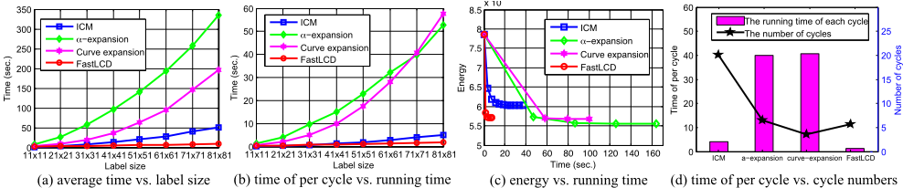
Synthetic data The computation time of optimizing of 2D label MRFs is greatly influenced by the label size of MRFs. To provide a detailed evaluation on different label sizes, we test FastLCD on the synthetic MRFs whose parameters are generated randomly. Following [Kumar and Torr, 2008], the data term ✓p(fp) are sampled uniformly from the interval [0↪ 10]. For the pairwise term, we use the function g(u↪ v)= k(u+v) and set k=1. In the experiments, we quantify the run time taken by the algorithms on MRFs with different label sizes that range from 11⇥11 to 81⇥81.
4.2 Performance analysis and comparison
We demonstrate the effectiveness of FastLCD and show the experimental analysis in this section. The performance of FastLCD is compared with several state-of-the-art methods, including ICM [Besag, 1986], ↵-expansion, ↵β-swap, curve expansion, BPS and TRWS.
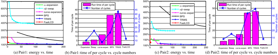
Efficiency Fig. 4 and Tab. 1 show the run time taken by different algorithms for image matching and optical flow. We see that FastLCD runs 6-7 times faster than ↵-expansion on image matching, and 5-8 times faster on optical flow estimation. FastLCD runs much faster because ↵-expansion requires m · n (♣X♣ =m, ♣Y♣ =n) moves in each cycle of iterations,
150%
100%
10s
0s
8.5 x 10 4
| Algorithm | Army | Mequon | Schefflera | Wooden | Grove | Urban |
|---|---|---|---|---|---|---|
| ICM | 135.3 | 106.3 | 92.3 | 135.7 | 132.4 | 145.4 |
| ↵-expansion | 167.6 | 192.3 | 148.6 | 128.2 | 315.8 | 323.9 |
| ↵β-swap | 523.5 | 625.3 | 296.3 | 317.6 | 561.2 | 589.6 |
| curve-expan. | 116.6 | 201.3 | 124.7 | 143.6 | 235.9 | 168.2 |
| BPS | 1491.0 | 1429.6 | 1544.8 | 1632.9 | 2332.7 | 2161.5 |
| TRWS | 1916.9 | 1819.9 | 1950.4 | 2080.8 | 2735.5 | 2780.7 |
| FastLCD | 34.4 | 65.8 | 56.1 | 44.8 | 91.8 | 55.3 |
| ICM | 490.6 | 590.9 | 408.0 | 430.5 | 442.2 | 340.9 |
| ↵-expansion | 265.8 | 525.3 | 360.8 | 656.1 | 993.4 | 578.1 |
| ↵β-swap | 2066.1 | 2276.4 | 2083.1 | 2376.5 | 2777.4 | 2709.8 |
| FastLCD | 69.2 | 113.3 | 62.4 | 92.3 | 125.6 | 131.4 |
while FastLCD only needs m+n+4 moves. As shown in Fig. 4(b) and (d), FastLCD takes much less time in each cycle than ↵-expansion. Meanwhile, we see that FastLCD and ↵-expansion take similar numbers of cycles to converge as shown in Fig. 4(b) and (d). Therefore, FastLCD offers a great speedup over ↵-expansion. Especially when the label space is huge, the advantage of FastLCD will be more obvious. As illustrated in Fig. 7, the run time of ↵-expansion increases rapidly as the label size increases. In contrast, the run time of FastLCD increases more slowly. For example, when the label size increases from 11⇥11 to 81⇥81, the run time of ↵- expansion increases more than 40 times (from 7.7s to 335.3s), while FastLCD increases less than 8 times (from 1.7s to 8.1s). We observe that FastLCD runs more than 40 times faster than ↵-expansion when the label space is 81⇥81. Thus, FastLCD benefits from the lower time complexity of O(m + n) per cycle.
From Fig. 7, we see that curve expansion also increase much more rapidly than FastLCD as the label size increases. From Fig. 4 and Tab. 1, we also observe FastLCD runs much faster than curve-expansion. This is because that curve-expansion needs to construct a huge graph and it takes a lot of time to solve the graph cuts in every cycle. As shown in Fig. 7(b),(d) and Fig. 4(b),(d), FastLCD takes much less time for each cycle than curve-expansion, while they take similar number of cycles in the optimization. For example, when the label set is 81 ⇥ 81, FastLCD (1.3s) runs more than 40 times faster than curve-expansion (57.6s) in each cycle of iterations.
From Fig. 4 and Tab. 1, we see that FastLCD runs about 45 times faster than BPS and 50 faster than TRWS. We did not compare FastLCD with BPS and TRWS on MRFs with a larger label set (such as the second group of experiments on optical flow estimation), because both BPS and TRWS require too much time to converge when the label size is huge. Compared with ↵β-swap, FastLCD also offers a great speedup, e.g., it runs about 30 times faster than ↵β-swap in the experiments of optical flow estimation. We see that FastLCD even runs faster than ICM, because it takes much fewer iterations to converge than ICM as shown in Fig. 7(d).
Performance Fig. 4 and Fig. 6 demonstrate the energies obtained from different algorithms on image matching and optical flow estimation. We see that FastLCD obtains similar energies compared to ↵-expansion and TRWS, and it obtains much lower energy than ICM and ↵β-swap. It can be seen that FastLCD yield competitive results on different types of energies including not only metric but also semimetric functions (Fig. 4(a),(c) and Fig. 6(c)), where the method of approximate moves is required in the optimization. The competitive results on smeimetric functions demonstrates the effectiveness of the approximate graph construction method described in Sec. 3.1.
Besides the energies, we also evaluate the quality of solutions obtained from the FastLCD algorithm. Fig. 5shows the solutions on image matching.From the figures, we observe that FastLCD yields comparable and similar solutions to the stateof-the-art algorithms including ↵-expansion, curve expansion and TRWS.
5 Conclusions
In this paper, we presented an efficient algorithm (called FastLCD) for the optimization of 2D label MRFs. The FastLCD utilizes the fact that the label set is two-dimensional, and optimizes the MRF energy by alternately performing label coordinate descents in horizontal, vertical and diagonal directions. The main advantage is that the FastLCD does not need to visit all the labels exhaustively as traditional algorithms, and it benefits from a lower time complexity of O(m+n) for each cycle. In the iterative moves, we propose an approximate graph construction to allow FastLCD to handle arbitrary semimetric energies. Moreover, we provide a theoretical guarantee for the approximate construction. The experimental results show that the FastLCD offers a great speedup over previous algorithms, while still yields competitive solutions.
Acknowledgments
This work is funded by the National Basic Research Program of China (Grant No. 2012CB316302), National Natural Science Foundation of China (Grant No. 61322209, 61403387, 61403388), the Strategic Priority Research Program of the Chinese Academy of Sciences (Grant XDA06040102). We thank Professor Philip Torr for his great help and valuable comments.
@inproceedings{ijcai2016p95,
  title     = {FastLCD: Fast Label Coordinate Descent for the Efficient Optimization of 2D Label MRFs},
  author    = {Liu, Kangwei and Zhang, Junge and Yang, Peipei and Huang, Kaiqi},
  booktitle = {Proceedings of the Twenty-Fifth International Joint Conference on
               Artificial Intelligence, {IJCAI-16}},
  publisher = {AAAI Press / International Joint Conferences on Artificial Intelligence},
  editor    = {Subbarao Kambhampati},
  pages     = {624--629},
  year      = {2016},
  month     = {7},
  url       = {https://ijcai.org/proceedings/2016/95},
}
TY - CPAPER TI - FastLCD: Fast Label Coordinate Descent for the Efficient Optimization of 2D Label MRFs AU - Liu, Kangwei AU - Zhang, Junge AU - Yang, Peipei AU - Huang, Kaiqi T2 - Proceedings of the Twenty-Fifth International Joint Conference on Artificial Intelligence, IJCAI-16 PB - AAAI Press / International Joint Conferences on Artificial Intelligence PY - 2016 SP - 624 EP - 629 UR - https://ijcai.org/proceedings/2016/95 ER -Copied
Machine-readable versions of this paper, for tools and AI agents:





