
Fast and Accurate Neural CRF Constituency Parsing
Proceedings of the Twenty-Ninth International Joint Conference on Artificial Intelligence. Main track. Pages 4046-4053.
https://doi.org/10.24963/ijcai.2020/560
Keywords
- Natural Language Processing: Tagging, chunking, and parsing
Abstract
Estimating probability distribution is one of the core issues in the NLP field.
However, in both deep learning (DL) and pre-DL eras, unlike the vast applications of linear-chain CRF in sequence labeling tasks, very few works have applied tree-structure CRF to constituency parsing, mainly due to the complexity and inefficiency of the inside-outside algorithm.
This work presents a fast and accurate neural CRF constituency parser.
The key idea is to batchify the inside algorithm for loss computation by direct large tensor operations on GPU, and meanwhile avoid the outside algorithm for gradient computation via efficient back-propagation.
We also propose a simple two-stage bracketing-then-labeling parsing approach to improve efficiency further.
To improve the parsing performance, inspired by recent progress in dependency parsing, we introduce a new scoring architecture based on boundary representation and biaffine attention, and a beneficial dropout strategy.
Experiments on PTB, CTB5.1, and CTB7 show that our two-stage CRF parser achieves new state-of-the-art performance on both settings of w/o and w/ BERT, and can parse over 1,000 sentences per second.
We release our code at https://github.com/yzhangcs/crfpar.
- [Akoury et al., 2019] Nader Akoury, Kalpesh Krishna, and Mohit Iyyer. Syntactically supervised transformers for faster neural machine translation. In Proceedings of ACL, pages 1269-1281, 2019.
- [Collins, 1997] Michael Collins. Three generative, lexi- calised models for statistical parsing. In Proceedings of ACL, pages 16-23, 1997.
- [Cross and Huang, 2016] James Cross and Liang Huang. Span-based constituency parsing with a structure-label system and provably optimal dynamic oracles. In Proceed- ings of EMNLP, pages 1-11, 2016.
- [Devlin et al., 2019] Jacob Devlin, Ming-Wei Chang, Ken- ton Lee, and Kristina Toutanova. BERT: Pre-training of deep bidirectional transformers for language understand- ing. In Proceedings of NAACL, pages 4171-4186, 2019.
- [Dozat and Manning, 2017] Timothy Dozat and Christo- pher D. Manning. Deep biaffine attention for neural de- pendency parsing. In Proceedings of ICLR, 2017.
- [Durrett and Klein, 2015] Greg Durrett and Dan Klein. Neu- ral CRF parsing. In Proceedings of ACL-IJCNLP, pages 302-312, 2015.
- [Eisner, 2016] Jason Eisner. Inside-outside and forward- backward algorithms are just backprop (tutorial paper). In Proceedings of WS, pages 1-17, 2016.
- [Finkel et al., 2008] Jenny Rose Finkel, Alex Kleeman, and Christopher D. Manning. Efficient, feature-based, condi- tional random field parsing. In Proceedings of ACL, pages 959-967, 2008.
- [Gaddy et al., 2018] David Gaddy, Mitchell Stern, and Dan Klein. What's going on in neural constituency parsers? an analysis. In Proceedings of NAACL, pages 999-1010, 2018.
- [Gómez-Rodríguez and Vilares, 2018] Carlos Gómez- Rodríguez and David Vilares. Constituent parsing as sequence labeling. In Proceedings of EMNLP, pages 1314-1324, 2018.
- [Jin et al., 2020] Lifeng Jin, Linfeng Song, Yue Zhang, Kun Xu, Wei yun Ma, and Dong Yu. Relation extraction ex- ploiting full dependency forests. In Proceedings of AAAI, 2020.
- [Kaplan et al., 2004] Ron Kaplan, Stefan Riezler, Tracy H. King, John T. Maxwell III, Alex Vasserman, and Richard Crouch. Speed and accuracy in shallow and deep stochas- tic parsing. In Proceedings of HLT-NAACL, pages 97-104, 2004.
- [Kitaev and Klein, 2018] Nikita Kitaev and Dan Klein. Con- stituency parsing with a self-attentive encoder. In Proceed- ings of ACL, pages 2676-2686, 2018.
- [Kitaev et al., 2019] Nikita Kitaev, Steven Cao, and Dan Klein. Multilingual constituency parsing with self- attention and pre-training. In Proceedings of ACL, pages 3499-3505, 2019.
- [Lample et al., 2016] Guillaume Lample, Miguel Balles- teros, Sandeep Subramanian, Kazuya Kawakami, and Chris Dyer. Neural architectures for named entity recogni- tion. In Proceedings of NAACL, pages 2475-2485, 2016.
- [Le and Zuidema, 2014] Phong Le and Willem Zuidema. The inside-outside recursive neural network model for de- pendency parsing. In Proceedings of EMNLP, pages 729- 739, 2014.
- [Li et al., 2019] Ying Li, Zhenghua Li, Min Zhang, Rui Wang, Sheng Li, and Luo Si. Self-attentive biaffine depen- dency parsing. In Proceedings of IJCAI, pages 5067-5073, 2019. IJCAI
- [Matsuzaki et al., 2005] Takuya Matsuzaki, Yusuke Miyao, and Jun'ichi Tsujii. Probabilistic CFG with latent annota- tions. In Proceedings of ACL, pages 75-82, 2005.
- [Peters et al., 2018] Matthew Peters, Mark Neumann, Mohit Iyyer, Matt Gardner, Christopher Clark, Kenton Lee, and Luke Zettlemoyer. Deep contextualized word representa- tions. In Proceedings of NAACL, pages 2227-2237, 2018.
- [Petrov and Klein, 2007] Slav Petrov and Dan Klein. Im- proved inference for unlexicalized parsing. In Proceedings of NAACL, pages 404-411, 2007.
- [Rush, 2020] Alexander M. Rush. Torch-struct: Deep struc- tured prediction library. arXiv:2002.00876, 2020.
- [Sagae and Lavie, 2005] Kenji Sagae and Alon Lavie. A classifier-based parser with linear run-time complexity. In Proceedings of IWPT, pages 125-132, 2005.
- [Shen et al., 2018] Yikang Shen, Zhouhan Lin, Athul Paul Jacob, Alessandro Sordoni, Aaron Courville, and Yoshua Bengio. Straight to the tree: Constituency parsing with neural syntactic distance. In Proceedings of ACL, pages 1171-1180, 2018.
- [Smith and Smith, 2007] David A. Smith and Noah A. Smith. Probabilistic models of nonprojective dependency trees. In Proceedings of EMNLP, pages 132-140, 2007.
- [Stern et al., 2017] Mitchell Stern, Jacob Andreas, and Dan Klein. A minimal span-based neural constituency parser. In Proceedings of ACL, pages 818-827, 2017.
- [Taskar et al., 2004] Ben Taskar, Dan Klein, Mike Collins, Daphne Koller, and Christopher Manning. Max-margin parsing. In Proceedings of EMNLP, pages 1-8, 2004.
- [Teng and Zhang, 2018] Zhiyang Teng and Yue Zhang. Two local models for neural constituent parsing. In Proceed- ings of COLING, pages 119-132, 2018.
- [Vilares et al., 2019] David Vilares, Mostafa Abdou, and Anders Søgaard. Better, faster, stronger sequence tag- ging constituent parsers. In Proceedings of NAACL, pages 3372-3383, 2019.
- [Wang and Chang, 2016] Wenhui Wang and Baobao Chang. Graph-based dependency parsing with bidirectional LSTM. In Proceedings of ACL, pages 2475-2485, 2016.
- [Wang et al., 2018] Xinyi Wang, Hieu Pham, Pengcheng Yin, and Graham Neubig. A tree-based decoder for neu- ral machine translation. In Proceedings of EMNLP, pages 4772-4777, 2018.
- [Zhang et al., 2020] Yu Zhang, Zhenghua Li, and Zhang Min. Efficient second-order TreeCRF for neural depen- dency parsing. In Proceedings of ACL, 2020.
- [Zhou and Zhao, 2019] Junru Zhou and Hai Zhao. Head- driven phrase structure grammar parsing on Penn treebank. In Proceedings of the ACL, pages 2396-2408, 2019.
- [Zhu et al., 2013] Muhua Zhu, Yue Zhang, Wenliang Chen, Min Zhang, and Jingbo Zhu. Fast and accurate shift-reduce constituent parsing. In Proceedings of ACL, pages 434- 443, 2013.
References were extracted automatically from the PDF and may contain errors.
Full text extracted automatically from the PDF; figures, tables and equations may differ. The PDF is the version of record.
1 Introduction
Given an input sentence, constituency parsing aims to build a hierarchical tree as depicted in Figure 1(a), where the leaf or terminal nodes correspond to input words and non-terminal nodes are constituents (e.g., VP3,5). As a fundamental yet challenging task in the natural language processing (NLP) field, constituency parsing has attracted a lot of research attention since large-scale treebanks were annotated, such as Penn Treebank (PTB), Penn Chinese Treebank (CTB), etc. Parsing outputs are also proven to be extensively useful for a wide range of downstream applications [Akoury et al., 2019; Wang et al., 2018].
∗Yu Zhang and Houquan Zhou make equal contributions to this work. Zhenghua Li is the corresponding author.
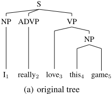
NP
I1
S∗
ADVP
really2
S
VP∗
love3
VP
NP∗
this4
NP
NP∗
game5
(b) CNF tree (left binarized)
Figure 1: Example constituency trees. Part-of-speech (POS) tags are not used as inputs in this work and thus excluded.
As one of the most influential works, Collins [1997] extends methods from probabilistic context-free grammars (PCFGs) to lexicalized grammars. Since then, constituency parsing has been dominated by such generative models for a long time, among which the widely used Berkeley parser adopts an unlexicalized PCFG with latent non-terminal splitting annotations [Matsuzaki et al., 2005; Petrov and Klein, 2007]. As for discriminative models, there exist two representative lines of research. The first line adopts the graphbased view based on dynamic programming decoding, using either local max-entropy estimation [Kaplan et al., 2004] or global max-margin training [Taskar et al., 2004]. The second group builds a tree via a sequence of shift-reduce actions based on greedy or beam decoding, known as the transitionbased view [Sagae and Lavie, 2005; Zhu et al., 2013].
Recently, constituency parsing has achieved significant progress thanks to the impressive capability of deep neural networks in context representation. Two typical and popular works are respectively the transition-based parser of Cross and Huang [2016] and the graph-based parser of Stern et al. [2017]. As discriminative models, the two parsers share several commonalities, both using 1) multi-layer BiLSTM as encoder; 2) minus features from BiLSTM outputs as span representations; 3) MLP for span scoring; 4) maxmargin training loss. Most works [Gaddy et al., 2018; Kitaev and Klein, 2018] mainly follow the two parsers and achieve much higher parsing accuracy than traditional nonneural models, especially with contextualized word representations trained with language modeling loss on large-scale unlabeled data [Peters et al., 2018; Devlin et al., 2019].
Despite the rapid progress, existing constituency parsing research suffers from two closely related drawbacks. First, parsing (also for training) speed is slow and can hardly satisfy the requirement of real-life systems. Second, the lack of explicitly modeling tree/subtree probabilities may hinder the effectiveness of utilizing parsing outputs. On the one hand, estimating probability distribution is one of the core issues in the NLP field [Le and Zuidema, 2014]. On the other hand, compared with unbounded tree scores, tree probabilities can better serve high-level tasks as soft features [Jin et al., 2020], and marginal probabilities of subtrees can support the more sophisticated Minimum Bayes Risk (MBR) decoding [Smith and Smith, 2007].
In fact, Finkel et al. [2008] and Durrett and Klein [2015] both propose CRF-based constituency parsing by directly modeling the conditional probability. However, both models are extremely inefficient due to the high time-complexity of the inside-outside algorithm for loss and gradient computation, especially the outside procedure. The issue becomes more severe in the DL era since all previous works perform the inside-outside computation on CPUs according to our knowledge and switching between GPU and CPU is expensive.
This work proposes a fast and accurate CRF constituency parser by substantially extending the graph-based parser of Stern et al. [2017]. The key contribution is that we batchify the inside algorithm for direct loss and gradient computation on GPU. Meanwhile, we find that the outside algorithm can be efficiently fulfilled by automatic backpropagation, which is shown to be equally efficient with the inside (forward) procedure, naturally verifying the great theoretical work of Eisner [2016]. Similarly, we batchify the Cocke-Kasami-Younger (CKY) algorithm for fast decoding.
In summary, we make the following contributions.
- We for the first time propose a fast and accurate CRF constituency parser for directly modeling (marginal) probabilities of trees and subtrees. The efficiency issue, which bothers the community for a long time, is well solved by elegantly batchifying the inside and CKY algorithms for direct computation on GPU.
- We propose a two-stage bracketing-then-labeling parsing approach that is more efficient and achieves slightly better performance than the one-stage method.
- We propose a new span scoring architecture based on span boundary representation and biaffine attention scoring, which performs better than the widely used minusfeature method. We also show that the parsing performance can be improved by a large margin via better parameter settings such as dropout configuration.
- Experiments on three English and Chinese benchmark datasets show that our proposed two-stage CRF parser achieves new state-of-the-art parsing performance under both settings of w/o and w/ BERT [Devlin et al., 2019]). In terms of parsing speed, our parser can parse over 1,000 sentences per second.
2 Two-stage CRF Parsing
Formally, given a sentence consisting of n words x = w0, . . . ,wn-1, a constituency parse tree, as depicted in Figure 1(a), is denoted as t, and (i, j, l) ∈ t is a constituent spanning wi...wj with a syntactic label l ∈ L. Alternatively, a tree can be factored into two parts, i.e., t = (y, l), where y is an unlabeled (a.k.a. bracketed) tree and l is a label sequence for all constituents in a certain order. Interchangeably, (3, 5, VP) is also denoted as VP3,5.
To accommodate the inside and CKY algorithms, we transform the original tree into those of Chomsky normal form (CNF) using the NLTK tool 1 , as shown in Figure 1(b). Particularly, consecutive unary productions such as Xi,j → Yi,j are collapsed into one X+Yi,j. We adopt left binarization since preliminary experiments show it is slightly superior to right binarization. After obtaining the 1-best tree via CKY decoding, the CNF tree is recovered into the n-ary form.
2.1 Model Definition
In this work, we adopt a two-stage bracketing-then-labeling framework for constituency parsing, which we show not only simplifies the model architecture but also improves efficiency, compared with the traditional one-stage approach adopted in previous works [Stern et al., 2017; Gaddy et al., 2018].
First stage: bracketing. Given x, the goal of the first stage is to find an optimal unlabeled tree y. The score of a tree is decomposed into the scores of all contained constituents.
Under CRF, the conditional probability is
where Z(x) is known as the normalization term, and T (x) is the set of legal trees.
Given all constituent scores s(i, j), we use the CKY algorithm to find the optimal tree ˆy.
Second stage: labeling. Given a sentence x and a tree y, the second stage independently predicts a label for each constituent (i, j) ∈ y.
Note that we use gold-standard unlabeled trees for loss computation during training. For a sentence of length n, all CNF trees contain the same 2n - 1 constituents. Therefore, this stage has a time complexity of O(n|L|).
Time complexity analysis. The CKY algorithm has a time complexity of O(n3 ). Therefore, the time complexity of our two-stage parsing approach is O(n3 +n|L|). In contrast, for the one-stage parsing approach, the CKY algorithm needs to determine the best label for all n2 spans and thus needs O(n3 + n2 |L|), where |L| is usually very large (e.g., 138 for English in Table 1).
2.2 Scoring Architecture
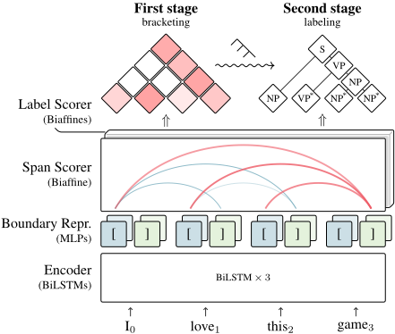
This subsection introduces the network architecture for scoring spans and labels, as shown in Figure 2, which mostly follows Stern et al. [2017] with two important modifications: 1) boundary representation and biaffine attention for score computation; 2) better parameter settings following Dozat and Manning [2017].
Inputs. For the ith word, its input vector ei is the concatenation of the word embedding and character-level representation:
where CharLSTM(wi) is the output vectors after feeding the character sequence into a BiLSTM layer [Lample et al., 2016]. Previous works show that replacing POS tag embeddings with CharLSTM(wi) leads to consistent improvement [Kitaev and Klein, 2018]. This can also simplify the model without the need of predicting POS tags (n-fold jack-knifing on training data).
BiLSTM encoder. We employ three BiLSTM layers over the input vectors for context encoding. We denote as fi and bi respectively the output vectors of the top-layer forward and backward LSTMs for wi.
In this work, we borrow most parameter settings from the dependency parser of Dozat and Manning [2017]. We find that the dropout strategy is very crucial for parsing performance, which differs from the vanilla implementation of Stern et al. [2017] in two aspects.
First, for each word wi, eword i and CharLSTM(wi) are dropped as a whole, either unchanged or becoming a 0 vector. If one vector is dropped into 0, the other is compensated with a ratio of 2. Second, the same LSTM layer shares the same dropout masks at different timesteps (words).
Boundary representation. For each word wi, we compose the context-aware word representation following Stern et al. [2017]. 2
The dimensions of hi is 800.
Instead of directly applying a single MLP to hi, we observe that a word must act as either left or right boundaries in all constituents in a given tree. Therefore, we employ two MLPs to make such distinction and obtain left and right boundary representation vectors.
The dimension d of rl/r i is 500. As pointed out by Dozat and Manning [2017], MLPs reduce the dimension of hi and, more importantly, detain only syntax-related information, thus alleviating the risk of over-fitting.
Biaffine scoring. Given the boundary representations, we score each candidate constituent (i, j) using biaffine operation over the left boundary representation of wi and the right boundary representation of wj .
where W ∈ Rd×d .
It is analogous to compute scores of constituent labels s(i, j, l). Two extra MLPs are applied to hi to obtain boundary representations ¯rl/r i (with dimension ¯ d). We then use |L| biaffines (R ¯ d× ¯ d ) to obtain all label scores. Since |L| is large, we use a small dimension ¯ d of 100 for ¯rl/r i (vs. 500 for rl/r i ) to reduce memory and computation cost.
Previous scoring method. Stern et al. [2017] use minus features of BiLSTM outputs as span representations [Wang and Chang, 2016; Cross and Huang, 2016] and apply MLPs to compute span scores.
We show that our new scoring method is clearly superior in the experiments.
2.3 Training Loss
For a training instance (x, y, l), The training loss is composed of two parts.
The first term is the sentence-level global CRF loss, trying to maximize the conditional probability:
where logZ(x) can be computed using the inside algorithm in O(n3 ) time complexity.
The second term is the standard constituent-level crossentropy loss for the labeling stage.
Algorithm 1 Batchified Inside Algorithm.
| 1: 2: | define: S ∈ Rn×n×B ✄ B is #sents in a batch initialize: all S:,: = 0 |
| 3: | for w = 1 to n do ✄ span width |
| 4: | Parallel computation on 0 ≤ i,j < n, r,0 ≤ b < B |
| 5: | Si,j=i+w = log ∑ i≤r<j exp (Si,r + Sr+1,j ) + s(i, j) |
| 6: | end for |
| 7: | return logZ |
7: return S0,n-1 ≡ logZ
3 Efficient Training and Decoding
This section describes how we perform efficient training and decoding via batchifying the inside and CKY algorithms for direct computation on GPU. We also show that the very complex outside algorithm can be avoided and fulfilled by the back-propagation process.
3.1 The Batchified Inside Algorithm
To compute logZ in Equation 11 and feature gradients, all previous works on CRF parsing [Finkel et al., 2008; Durrett and Klein, 2015] explicitly perform the inside-outside algorithm on CPUs. Unlike linear-chain CRF, it seems very difficult to batchify tree-structure algorithms.
In this work, we find that it is feasible to propose a batchified version of the inside algorithm, as shown in Algorithm 1. The key idea is to pack the scores of same-width spans for all instances in the data batch into large tensors. This allows us to do computation and aggregation simultaneously via efficient large tensor operation. Since computation for all 0 ≤ i,j < n, r,0 ≤ b < B is performed in parallel on GPU, the algorithm only needs O(n) steps. Our code will give more technical details.
3.2 Outside via Back-propagation
Traditionally, the outside algorithm is considered as indispensable for computing marginal probabilities of subtrees, which further compose feature gradients. In practice, the outside algorithm is more complex and at least twice slower than the inside algorithm. Though possible, it is more complicated to batchify the outside algorithm. Fortunately, this issue is erased in the deep learning era since the back-propagation procedure is designed to obtain gradients. In fact, Eisner [2016] proposes a theoretical discussion on the equivalence between the back-propagation and outside procedures.
Since we use a batchified inside algorithm during the forward phase, the back-propagation is conducted based on large tensor computation, which is thus equally efficient.
It is also noteworthy that, by setting the loss to logZ and performing back-propagation, we can obtain the marginal probabilities of spans (i, j), which is exactly the corresponding gradients.
2 Our preliminary experiments show that fi ⊕bi+1 achieves consistent improvement over fi ⊕bi. The possible reason may be that both fi and bi use ei as input and thus provide redundant information.
| #Train | #Dev | #Test | #labels | ||
|---|---|---|---|---|---|
| original | CNF | ||||
| PTB | 39,832 | 1,700 | 2,416 | 26 | 138 |
| CTB5.1 | 18,104 | 352 | 348 | 26 | 162 |
| CTB7 | 46,572 | 2,079 | 2,796 | 28 | 265 |
Marginal probabilities are also useful in many subsequent NLP tasks as soft features. Please refer to Eisner [2016] for more details.
3.3 Decoding
As mentioned above, we employ the CKY algorithm to obtain the 1-best tree during the parsing phase, as shown in Equation 3. The CKY algorithm is almost identical to the inside algorithm except for replacing the sum-product with a max product (refer to Line 5 in Algorithm 1) and thus can also be efficiently batchified.
To perform MBR decoding, we simply replace the span scores s(i, j) with the marginal probabilities p((i, j) | x) in Equation 1 and 3. However, we find this has little influence on parsing performance.
4 Experiments
Data. We conduct experiments on three English and Chinese datasets. The first two datasets, i.e., PTB and CTB5.1, are widely used in the community. We follow the conventional train/dev/test data split. Considering that both CTB5.1dev/test only have about 350 sentences, we also use the larger CTB7 for more robust investigations, following the data split suggested in the official manual. Table 1 shows the data statistics. We can see that CNF introduces many new constituent label types, most (about 75%) of which are from the collapsing process of consecutive unary rules.
Evaluation. As mentioned earlier, we convert 1-best CNF trees into n-ary trees after parsing for evaluation. Here, it may be useful to mention a small detail. The predicted 1best CNF tree may contain inconsistent productions since the decoding algorithm does not have such constraints. Taking Figure 1(b) as an example, the model may output VP3,5 → PP∗3,3 NP4,5, where VP is incompatible with PP∗ . During the n-ary post-processing, we simply ignore the concrete label string PP before the "∗" symbol. In view of this, performance may be slightly improved by adding such constraints during decoding.
We use the standard constituent-level labeled precision, recall, F-score (P/R/F) as the evaluation metrics with the EVALB tool 3 . Specifically, a predicted constituent such as VP3,5 is considered correct if it also appears in the goldstandard tree. 4
3 https://nlp.cs.nyu.edu/evalb
| PTB | CTB5.1 | CTB7 | |||||||
|---|---|---|---|---|---|---|---|---|---|
| P | R | F | P | R | F | P | R | F | |
| Max-margin (one-stage) | 93.70 | 93.73 | 93.72 | 90.60 | 90.48 | 90.54 | 86.85 | 86.08 | 86.47 |
| CRF (one-stage) | 93.44 | 93.75 | 93.60 | 91.08 | 90.98 | 91.03 | 87.10 | 86.75 | 86.93 |
| CRF (two-stage) | 93.77 | 93.96 | 93.86 | 90.91 | 91.09 | 91.00 | 87.27 | 87.00 | 87.13 |
| w/o MBR | 93.75 | 93.85 | 93.80 | 90.93 | 91.10 | 91.02 | 87.21 | 86.89 | 87.05 |
| minus features | 93.40 | 93.35 | 93.37 | 90.60 | 90.51 | 90.56 | 86.96 | 86.24 | 86.60 |
| vanilla dropout | 92.80 | 93.00 | 92.90 | 89.68 | 89.68 | 89.68 | 85.55 | 85.54 | 85.54 |
Parameter settings. We directly adopt the same hyperparameter settings of the dependency parser of Dozat and Manning [2017] without further tuning. The only difference is the use of CharLSTM word representations instead of POS tag embeddings. The dimensions of char embedding, word embedding, and CharLSTM outputs are 50, 100, 100, respectively. All dropout ratios are 0.33. The mini-batch size is 5,000 words. The training process continues at most 1,000 epochs and is stopped if the peak performance on dev data does not increase in 100 consecutive epochs.
4.1 Model Comparison on Dev Data
We conduct the model study on dev data from two aspects: 1) CRF vs. max-margin training loss; 2) two-stage vs. one-stage parsing. The first three lines of Table 2 shows the results. The three models use the same scoring architecture and parameters. Following previous practice [Stern et al., 2017], onestage models use only scores of labeled constituents s(i, j, l). In order to verify the effectiveness of the two-stage parsing, we also list the results of "CRF (one-stage)", which directly scores labeled constituents.
As discussed in the last paragraph of Section 2.1, the inside and CKY algorithms become a bit more complicated for the one-stage parser that two-stage.
From the first two rows, we can see that under the onestage parsing framework, the CRF loss leads to similar performance on English but consistently outperforms the maxmargin loss by about 0.5 F-score on both Chinese datasets. The max-margin loss has one extra hyper-parameter, namely the margin value, which is set to 1 according to preliminary results on English and not tuned on Chinese for simplicity. We suspect that the performance on Chinese with maxmargin loss may be improved with more tuning. Overall, we can conclude that the two training loss settings achieve very close performance, and CRF has an extra advantage of probabilistic modeling.
4 Since some researchers may implement their own evaluation scripts, some details about EVALB need to be clarified for fair comparison: 1) Empty constituents like {-NONE-} are removed during data pre-processing. 2) Root constituents ({TOP, S1} for English and an empty string for Chinese) are ignored for evaluation. 3) Constituents spanning a English punctuation mark like {:, ", ", ., ?, !} are also ignored. Please note that Chinese punctuation marks are evaluated as normal words. 4) Some label sets like {ADVP, PRT} are regarded as equivalent.
| Sents/sec | |
|---|---|
| Petrov and Klein [2007] (Berkeley Parser) | 6 |
| Zhu et al. [2013] (ZPar) | 90 |
| Stern et al. [2017] | 76 |
| Shen et al. [2018] | 111 |
| Kitaev and Klein [2018] | 332 |
| G´omez-Rodr´ıguez and Vilares [2018] | 780 |
| CRF (one-stage) | 990 |
| CRF (two-stage) w/ MBR | 743 |
| CRF (two-stage) w/o MBR | 1092 |
Comparing the second and third rows, the two CRF parsers achieve nearly the same performance on CTB5.1 and the twostage parser achieves modest improvement over the one-stage parser by about 0.2 F-score on both PTB and CTB7. Therefore, we can conclude that our proposed two-stage parsing approach is superior in simplicity and efficiency (see Table 3) without hurting performance.
4.2 Ablation Study on Dev Data
To gain insights into the contributions of individual components in our proposed framework, we then conduct the ablation study by undoing one component at a time. Results are shown in the bottom four rows of Table 2.
Impact of MBR decoding. By default, we employ CKY decoding over marginal probabilities, a.k.a. MBR decoding. The "w/o MBR" row presents the results of performing decoding over span scores. Such comparison is very interesting since it is usually assumed that MBR decoding is theoretically superior to vanilla decoding. However, the results clearly show that the two decoding methods achieve nearly identical performance.
Impact of scoring architectures. In order to measure the effectiveness of our new scoring architecture, we revert the biaffine scorers to the "minus features" method adopted by Stern et al. [2017] (refer to Equation 9). It is clear that our proposed scoring method is superior to the widely used minus-feature method, and achieves a consistent and substantial improvement of about 0.5 F-score on all three datasets.
| PTB | CTB5.1 | CTB7 | |||||||
|---|---|---|---|---|---|---|---|---|---|
| P | R | F | P | R | F | P | R | F | |
| Stern et al. [2017] | 92.98 | 90.63 | 91.79 | - | - | - | - | - | - |
| Gaddy et al. [2018] | 92.41 | 91.76 | 92.08 | - | - | - | - | - | - |
| Kitaev and Klein [2018] | 93.90 | 93.20 | 93.55 | 88.09 | 86.78 | 87.43 | - | - | - |
| G´omez-Rodr´ıguez and Vilares [2018] | - | - | 90.00 | - | - | 84.40 | - | - | - |
| Shen et al. [2018] | 92.00 | 91.70 | 91.80 | 86.60 | 86.40 | 86.50 | - | - | - |
| Teng and Zhang [2018] | 92.50 | 92.20 | 92.40 | 87.50 | 87.10 | 87.30 | - | - | - |
| Vilares et al. [2019] | - | - | 90.60 | - | - | 85.61 | - | - | - |
| Zhou and Zhao [2019] w/ pretrained | 93.92 | 93.64 | 93.78 | 89.70 | 89.09 | 89.40 | - | - | - |
| Ours | 93.84 | 93.58 | 93.71 | 89.18 | 89.03 | 89.10 | 87.66 | 87.21 | 87.43 |
| Ours w/ pretrained | 94.23 | 94.02 | 94.12 | 89.71 | 89.89 | 89.80 | 88.84 | 88.36 | 88.60 |
| Kitaev and Klein [2018] w/ ELMo | 95.40 | 94.85 | 95.13 | - | - | - | - | - | - |
| Kitaev et al. [2019] w/ BERT | 95.73 | 95.46 | 95.59 | 91.96 | 91.55 | 91.75 | - | - | - |
| Ours w/ BERT | 95.85 | 95.53 | 95.69 | 92.51 | 92.04 | 92.27 | 91.73 | 91.38 | 91.55 |
Impact of dropout strategy. We keep other model settings unchanged and only replace the dropout strategy borrowed from Dozat and Manning [2017] with the vanilla dropout strategy adopted by Stern et al. [2017]. This leads to a very large and consistent performance drop of 0.96, 1.39 and 1.59 in F-score on the three datasets, respectively. Kitaev and Klein [2018] replaced BiLSTMs with a self-attention encoder in Stern et al. [2017] and achieved a large improvement of 1.0 F-score by separating content and position attention. Similarly, this work shows that the BiLSTM-based parser can be very competitive with proper parameter settings.
4.3 Speed Comparison
Table 3 compares different parsing models in terms of parsing speed. Our models are both run on a machine with Intel Xeon E5-2650 v4 CPU and Nvidia GeForce GTX 1080 Ti GPU. Berkeley Parser and ZPar are two representative nonneural parsers without access to GPU. Stern et al. [2017] employ max-margin training and perform CKY-like decoding on CPUs. Kitaev and Klein [2018] use a self-attention encoder and perform decoding using Cython for acceleration.
We can see that our one-stage CRF parser is much more efficient than previous parsers by directly performing decoding on GPU. Our two-stage parser can parse 1,092 sentences per sentence, which is three times faster than Kitaev and Klein [2018]. Of course, it is noteworthy that those parsers [Stern et al., 2017; Kitaev and Klein, 2018] may be equally efficient by adopting our batchifying techniques.
The parser of G´omez-Rodr´ıguez and Vilares [2018] is also very efficient by treating parsing as a sequence labeling task. However, the parsing performance is much lower, as shown in Table 4.
The two-stage parser is only about 10% faster than the onestage counterpart. The gap seems small considering the significant difference in time complexity as discussed (see Section 2.1). The reason is that the two parsers share the same encoding and scoring components, which consume a large portion of the parsing time.
Using MBR decoding requires an extra run of the inside and back-propagation algorithms for computing marginal probabilities, and thus is less efficient. As shown in Table 2, the performance gap is very slight between w/ and w/o MBR.
4.4 Results and Comparison on Test Data
Table 4 shows the final results on the test datasets under two settings, i.e., w/o and w/ ELMo/BERT.
Most previous works do not use pretrained word embedding but use randomly initialized ones instead, except for Zhou and Zhao [2019], who use Glove for English and structured skip-gram embeddings. For pretrained word embeddings, we use Glove (100d) for English PTB 5 , and adopt the embeddings of Li et al. [2019] trained on Gigaword 3rd Edition for Chinese. It is clear that our parser benefits substantially from the pretrained word embeddings. 6
We also make comparisons with recent related works on constituency parsing, as discussed in Section 5. We can see that our BiLSTM-based parser outperforms the basic Stern et al. [2017] by a very large margin, mostly owing to the new scoring architecture and better dropout settings. Compared with the previous state-of-the-art self-attentive parser [Kitaev and Klein, 2018], our parser achieves an absolute improvement of 0.16 on PTB and 1.67 on CTB5.1 without any language-specific settings.
The CTB5.1 results of Zhou and Zhao [2019] is obtained by rerunning their released code using predicted POS tags. We follow their descriptions 7 to produce the POS tags. It is noteworthy that their reported results accidentally use gold POS tags on CTB5.1, which is confirmed after several turns of email communication. We are grateful for their patience
5 https://nlp.stanford.edu/projects/glove
7 https://github.com/DoodleJZ/HPSG-Neural-Parser and help. We reran their released code using gold POS tags, and got 92.14 in F-score on CTB5-test, very close to the results reported in their paper. Our parser achieves 92.66 Fscore with gold POS tags. Another detail about their paper should be clarified: for dependency parsing on Chinese, they adopt two different data split settings, both using Stanford dependencies 3.3.0 and gold POS tags.
6 We have also tried the structured skip-gram embeddings kindly shared by Zhou and Zhao [2019] for Chinese, and achieved similar performance by using our own embeddings.
The bottom three rows list the results under the setting of using ELMo/BERT. We use bert-large-cased 8 (24 layers, 1024 dimensions, 16 heads) for PTB following Kitaev et al. [2019], and bert-base-chinese (12 layers, 768 dimensions, 12 heads) for CTB. It is clear that using BERT representations can help our parser by a very large margin on all datasets. Our parser also outperforms the multilingual parser of Kitaev et al. [2019], which uses extra multilingual resources. In summary, we can conclude that our parser achieves state-of-theart performance in both languages and both settings.
5 RelatedWorks
Because of the inefficiency issue, there exist only a few previous works on CRF constituency parsing. Finkel et al. [2008] propose the first non-neural feature-rich CRF constituency parser. Durrett and Klein [2015] extend the work of Finkel et al. [2008] and use a feedforward neural network with nonlinear activation for scoring anchored production rules. Both works perform explicit inside-outside computations on CPUs and suffer from a severe inefficiency issue.
This work is built on the high-performance modern neural parser based on a BiLSTM encoder [Stern et al., 2017], which first applies minus features [Cross and Huang, 2016] for span scoring to graph-based constituency parsing. Several recent works follow Stern et al. [2017]. Gaddy et al. [2018] try to analyze what and how much context is implicitly encoded by BiLSTMs. Kitaev and Klein [2018] replace twolayer BiLSTM with self-attention layers and find considerable improvement via separated content and position attending. In contrast, this work shows that the parser of Stern et al. [2017] outperforms Kitaev and Klein [2018] by properly configuring BiLSTMs such as the dropout strategy (see Table 2). Please also kindly notice that Kitaev and Klein [2018] use very large word embeddings.
Batchification is straightforward and well-solved for sequence labeling tasks, as shown in the implementation of NCRF++ 9 . However, very few works turned sight to treestructures. In a slightly earlier work, we for the first time propose to batchify tree-structured inside and Viterbi (Eisner) computation for GPU acceleration for the dependency parsing [Zhang et al., 2020]. This work is an extension to the constituency parsing with different inside and Viterbi (CKY) algorithms.
As an independent and concurrent work to ours, TorchStruct 10 , kindly brought up by a reviewer, has also implemented batchified TreeCRF algorithms for constituency parsing [Rush, 2020]. However, Torch-Struct aims to provide general-purpose basic implementations for structure prediction algorithms. In contrast, we work on sophisticated parsing models, and aim to advance the state-of-the-art CRF constituency parsing in both accuracy and efficiency.
8 https://github.com/huggingface/transformers
9 https://github.com/jiesutd/NCRFpp
10 https://github.com/harvardnlp/pytorch-struct
Meanwhile, there is a recent trend of extremely simplifying the constituency parsing task without explicit structural consideration or the use of CKY decoding. G´omez-Rodr´ıguez and Vilares [2018] propose a sequence labeling approach for constituency parsing by designing a complex tag encoding tree information for each input word. Vilares et al. [2019] further enhance the sequence labeling approach via several augmentation strategies such as multi-task learning and policy gradients. Shen et al. [2018] propose to predict a scalar distance in the gold-standard parse tree for each neighboring word pairs and employ bottom-up greedy search to find an optimal tree. However, all the above works lag behind the mainstream approaches by a large margin in terms of parsing performance.
6 Conclusions
In this work, we propose a fast and accurate neural CRF constituency parser. We show that the inside and CKY algorithms can be effectively batchified to accommodate direct large tensor computation on GPU, leading to dramatic efficiency improvement. The back-propagation procedure is equally efficient and erases the need for the outside algorithm for gradient computation. Experiments on three English and Chinese benchmark datasets lead to several promising findings. First, the simple two-stage bracketing-then-labeling approach is more efficient than one-stage parsing without hurting performance. Second, our new scoring architecture achieves higher performance than the previous method based on minus features. Third, the dropout strategy we introduce can improve parsing performance by a large margin. Finally, our proposed parser achieves new state-of-the-art performances with a parsing speed of over 1,000 sentences per second.
Acknowledgments
The authors would like to thank the anonymous reviewers for their helpful comments. This work was supported by National Natural Science Foundation of China (Grant No. 61525205, 61876116) and a Project Funded by the Priority Academic Program Development (PAPD) of Jiangsu Higher Education Institutions.
@inproceedings{ijcai2020p560,
  title     = {Fast and Accurate Neural CRF Constituency Parsing},
  author    = {Zhang, Yu and Zhou, Houquan and Li, Zhenghua},
  booktitle = {Proceedings of the Twenty-Ninth International Joint Conference on
               Artificial Intelligence, {IJCAI-20}},
  publisher = {International Joint Conferences on Artificial Intelligence Organization},
  editor    = {Christian Bessiere},
  pages     = {4046--4053},
  year      = {2020},
  month     = {7},
  note      = {Main track},
  doi       = {10.24963/ijcai.2020/560},
  url       = {https://doi.org/10.24963/ijcai.2020/560},
}
TY - CPAPER TI - Fast and Accurate Neural CRF Constituency Parsing AU - Zhang, Yu AU - Zhou, Houquan AU - Li, Zhenghua T2 - Proceedings of the Twenty-Ninth International Joint Conference on Artificial Intelligence, IJCAI-20 PB - International Joint Conferences on Artificial Intelligence Organization PY - 2020 SP - 4046 EP - 4053 DO - 10.24963/ijcai.2020/560 UR - https://doi.org/10.24963/ijcai.2020/560 ER -Copied
Machine-readable versions of this paper, for tools and AI agents:





