
RHash: Robust Hashing via L_infinity-norm Distortion
Proceedings of the Twenty-Sixth International Joint Conference on Artificial Intelligence. Main track. Pages 1386-1394.
https://doi.org/10.24963/ijcai.2017/192
Keywords
- Machine Learning: Machine Learning
- Natural Language Processing: Information Retrieval
Abstract
Hashing is an important tool in large-scale machine learning. Unfortunately, current data-dependent hashing algorithms are not robust to small perturbations of the data points, which degrades the performance of nearest neighbor (NN) search. The culprit is the minimization of the L_2-norm, average distortion among pairs of points to find the hash function. Inspired by recent progress in robust optimization, we develop a novel hashing algorithm, dubbed RHash, that instead minimizes the L_1-norm, worst-case distortion among pairs of points. We develop practical and efficient implementations of RHash that couple the alternating direction method of multipliers (ADMM) framework with column generation to scale well to large datasets. A range of experimental evaluations demonstrate the superiority of RHash over ten state-of-the-art binary hashing schemes. In particular, we show that RHash achieves the same retrieval performance as the state-of-the-art algorithms in terms of average precision while using up to 60% fewer bits.
- [Boyd et al., 2011] S. Boyd, N. Parikh, E. Chu, B. Peleato, and J. Eckstein. Distributed optimization and statistical learning via the alternating direction method of multipli- ers. Found. Trends Mach. Learn., 3(1):1-122, Jan. 2011.
- [Chatterjee and Hadi, 2009] S. Chatterjee and A. S. Hadi. Sensitivity Analysis in Linear Regression, volume 327.
- [Dantzig and Wolfe, 1960] G. B. Dantzig and P. Wolfe. De- composition principle for linear programs. Operations Re- search, 8(1):101-111, Feb. 1960.
- [Datar et al., 2004] M. Datar, N. Immorlica, P. Indyk, and V. S. Mirrokni. Locality-sensitive hashing scheme based on p-stable distributions. In Proc. Annu. Symp. Comput. Geometry, pages 253-262, June 2004.
- [Du and Pardalos, 2013] D. Du and P. M. Pardalos. Minimax and Applications, volume 4. Springer, 2013.
- [Hartley and Schaffalitzky, 2004] R. Hartley and F. Schaffal- itzky. L ∞ minimization in geometric reconstruction prob- lems. In Proc. Conf. Comput. Vision Pattern Recogn. (CVPR), pages 504-509, June 2004.
- [He et al., 2012] J. He, S. Kumar, and S. Chang. On the diffi- culty of nearest neighbor search. In Proc. Int. Conf. Mach. Learn., pages 1127-1134, June 2012.
- [Hegde et al., 2015] C. Hegde, A. C. Sankaranarayanan, W. Yin, and R. G. Baraniuk. Numax: A convex approach for learning near-isometric linear embeddings. IEEE Trans. Signal Process., 63(22):6109-6121, Nov. 2015.
- [Heo et al., 2012] J. Heo, Y. Lee, J. He, S. Chang, and S. Yoon. Spherical hashing. In Proc. Conf. Comput. Vi- sion Pattern Recogn., pages 2957-2964, June 2012.
- [Indyk and Motwani, 1998] P. Indyk and R. Motwani. Ap- proximate nearest neighbors: Towards removing the curse of dimensionality. In Proc. Annu. Symp. Theory Comput., pages 604-613, May 1998.
- [Jégou et al., 2012] H. Jégou, T. Furon, and J. Fuchs. Anti- sparse coding for approximate nearest neighbor search. In Proc. Intl. Conf. Acoustics Speech Signal Process. (ICASSP), pages 2029-2032. IEEE, 2012.
- [Jiang and Li, 2015] Q. Y. Jiang and W. J. Li. Scalable graph hashing with feature transformation. In Proc Intl. Joint Conf. Artif. Intell., Sep. 2015. IJCAI
- [Kong and Li, 2012] W. Kong and W. Li. Isotropic hashing. In Adv. Neural Info. Process. Syst., pages 1646-1654, Dec. 2012.
- [Kulis and Darrell, 2009] B. Kulis and T. Darrell. Learning to hash with binary reconstructive embeddings. In Adv. Neural Inf. Process. Syst., pages 1042-1050, Dec. 2009.
- [LeCun and Cortes, 1998] Y. LeCun and C. Cortes. The MNIST database of handwritten digits, 1998.
- [Ledoux and Talagrand, 1991] M. Ledoux and M. Tala- grand. Probability in Banach Spaces: Isoperimetry and Processes. Springer-Verlag, 1991.
- [Liu et al., 2011] W. Liu, J. Wang, S. Kumar, and S. Chang. Hashing with graphs. In Proc. Intl. Conf. Mach. Learn., pages 1-8, July 2011.
- [Lowe, 2004] D. Lowe. Distinctive image features from scale-invariant keypoints. Int. J. Comput. Vision, 60(2):91-110, Nov. 2004.
- [Lv et al., 2007] Q. Lv, W. Josephson, Z. Wang, M. Charikar, and K. Li. Multi-probe lsh: efficient indexing for high- dimensional similarity search. In Proc. Int. Conf. Very Large databases, pages 950-961, Sep. 2007.
- [Nesterov, 2007] Y. Nesterov. Gradient methods for mini- mizing composite objective function. Technical report, Université Catholique de Louvain, Sep. 2007.
- [Norouzi and Fleet, 2011] M. Norouzi and D. J. Fleet. Min- imal loss hashing for compact binary codes. In Proc. Int. Conf. on Mach. Learn., pages 353-360, June 2011.
- [Plan and Vershynin, 2014] Y. Plan and R. Vershynin. Di- mension reduction by random hyperplane tessellations. Discrete Comput. Geom., 51(2):438-461, Mar. 2014.
- [Snavely et al., 2006] N. Snavely, S. Seitz, and R. Szeliski. Photo tourism: Exploring photo collections in 3D. ACM Trans. Graphics, 25(3):835-846, July 2006.
- [Studer et al., 2014] C. Studer, T. Goldstein, W. Yin, and R. G. Baraniuk. Democratic representations. arXiv preprint arXiv:1401.3420, 2014.
- [Torralba et al., 2008] A. Torralba, R. Fergus, and Y. Weiss. Small codes and large image databases for recognition. In Proc. Conf. Comput. Vision Pattern Recogn., pages 1-8, June 2008.
- [Wainwright, 2009] M. J. Wainwright. Sharp thresholds for high-dimensional and noisy sparsity recovery using ℓ 1 - constrained quadratic programming (Lasso). IEEE Trans. Info. Theory, 55(5):2183-2202, May 2009.
- [Wang et al., 2014] J. Wang, H. T. Shen, J. Song, and J. Ji. Hashing for similarity search: A survey. arXiv preprint arXiv:1408.2927, 2014.
- [Wang et al., 2016] Z. Wang, Y. Yang, S. Chang, Q. Ling, and T. S. Huang. Learning a deep ℓ ∞ encoder for hashing. In Proc. Intl. Joint Conf. Artif. Intell., pages 2174-2180. AAAI Press, 2016. IJCAI
- [Weiss et al., 2009] Y. Weiss, A. Torralba, and R. Fergus. Spectral hashing. In Adv. Neural Inf. Process. Syst., pages 1753-1760, Dec. 2009.
- [Weiss et al., 2012] Y. Weiss, R. Fergus, and A. Torralba. Multidimensional spectral hashing. In European Conf. Comput. Vision, pages 340-353, Oct. 2012.
- [Wen et al., 2010] Z. Wen, W. Yin, D. Goldfarb, and Y. Zhang. A fast algorithm for sparse reconstruction based on shrinkage, subspace optimization, and continuation. SIAM J. Sci. Comput., 32(4):1832-1857, June 2010.
- [Xu et al., 2009] H. Xu, C. Caramanis, and S. Mannor. Ro- bustness and regularization of support vector machines. J. Mach. Learn. Research, 10:1485-1510, 2009.
- [Yu et al., 2014] F. X. Yu, S. Kumar, Y. Gong, and S. Chang. Circulant binary embedding. In Proc. Int. Conf. Mach. Learn., pages 946-954, June 2014.
References were extracted automatically from the PDF and may contain errors.
Full text extracted automatically from the PDF; figures, tables and equations may differ. The PDF is the version of record.
1 Introduction
Hashing, one of the primitive operations in large-scale machine learning systems, seeks a low-dimensional binary embedding of a high-dimensional dataset. Such a binary embedding can increase the computational efficiency of a variety of tasks, including nearest neighbor (NN) search.
The embedding of high-dimensional data into short binary codes naturally distorts the set of top NNs of each data point. To minimize this distortion, a range of hashing schemes have been developed. The simplest, random projection, projects the data onto a lower-dimensional random subspace and then quantizes to binary values. Random projection belongs to the family of probabilistic, locality sensitive hashing (LSH) algorithms that guarantee the preservation of the set of NN points with small distortion [Datar et al., 2004]. The cost, however, is that LSH requires an impractically high number of bits to index real-world, large-scale datasets [Lv et al., 2007]. In response, data-dependent binary hashing algorithms have been developed that require significantly fewer bits; see [Wang et al., 2014] for a survey.
Data-dependent hashing algorithms learn a hash function by minimizing a measure of distortion between certain pairs of data points [Weiss et al., 2009; 2012]. For the task of NN search, it is sufficient to control the pairwise distortion among the NNs of each point plus a few additional points [Kulis and Darrell, 2009]. Given a pair of data points (xi, xj) in the ambient space and their corresponding embedded binary codes (hi, hj) in the Hamming space, define the pairwise distortion function δij = L(xi, xj ; hi, hj), where L(·) is a chosen loss function. The lion's share of data-dependent hashing algorithms use an ℓ2-norm loss function, which minimizes the average of the square of pairwise distortions ‖δ‖22 = ∑(i,j)∈Ω δ2 ij over a set of selected pairs of points Ω [Jiang and Li, 2015; Kong and Li, 2012; Kulis and Darrell, 2009; Liu et al., 2011; Weiss et al., 2009; 2012].
Unfortunately, the loss functions employed by the hashing community to date, including the ℓ2-norm loss, are not robust to perturbations of the data points. Indeed, the ℓ2norm average distortion is well-known to be sensitive to small disturbances and noise [Chatterjee and Hadi, 2009]. In this paper, we argue that alternative norms, in particular the ℓ∞- norm (which measures worst-case distortion) [Du and Pardalos, 2013; Hartley and Schaffalitzky, 2004; Xu et al., 2009], are more robust to small perturbations and thus more appropriate for designing data-dependent hash functions.
To elucidate the strong effect of the loss function on the robustness of a hashing function, we compare the hash functions learned using the ℓ2- and ℓ∞-norm losses on a subset of the MNIST dataset of handwritten digit images [LeCun and Cortes, 1998]. For visualization purposes, we project the data points onto the first two principal components and compute the optimal 1-dimensional binary embeddings generated by minimizing the ℓ2-norm distortion and the ℓ∞-norm distortion ‖δ‖∞ = max(i,j)∈Ω |δij| with |Ω| = 50. Figure 1(a) shows the ℓ2- and ℓ∞-optimal embeddings that we learned from a grid search. Figure 1(b) summarizes an experiment where we add a small amount of white Gaussian noise to each data point before computing the optimal embeddings. We see that the ℓ2-optimal embedding is increasingly less robust than the ℓ∞-optimal embedding as the amount of noise grows.
The robustness of the ℓ∞-optimal embedding translates directly to improved NN preservation. Continuing the MNIST example from above but with no added noise, Figure 1(c) illustrates that the top-5 NNs of the query point q are severely damaged by the ℓ2-optimal embedding but are left unscathed by the ℓ∞-optimal embedding. Figure 1(d) provides some insight into the reason. The ℓ2-norm (average distortion) optimal embedding does not preserve some of the distances between the digits "3", "5", and "9" and the digit "8" and thus projects some of them into the same neighborhood close to q. In contrast, the ℓ∞-norm (worst-case distortion) optimal embedding preserves these harder distances and thus preserves the set of original NNs of q with minimal distortion.
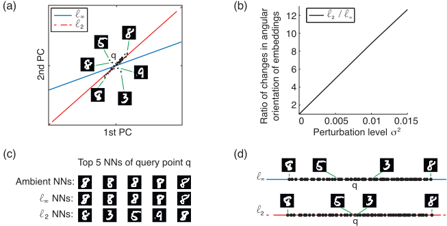
Inspired by the robustness of the ℓ∞-norm distortion [Du and Pardalos, 2013; Hartley and Schaffalitzky, 2004; Xu et al., 2009], we propose Robust Hashing (RHash), the first hashing algorithm that learns robust binary hash codes by minimizing the ℓ∞-norm of the pairwise distances vector ‖δ‖∞ = max(i,j)∈Ω |dH(hi, hj) - d(xi, xj)|, where d and dH denote the Euclidean and Hamming distances, respectively. The robustness of ℓ∞-norm distortion stems from its dependence on only the pairwise distortions that are hardest to preserve. As long as the hardest pairwise distortions are not affected, small perturbations do not alter the outcome of the embedding. In other words, in the NN retrieval task, where we only care about the distortions of NN pairs, the hardest pair to preserve is the deal-breaker. We emphasize that the worst-case distorted NN pair (under an embedding) is the hardest NN pair to be preserved and not the farthest pair nor a pair of outliers.
1.1 Contributions
We make four distinct contributions in this paper. First, conceptually, we advocate minimizing the more robust worstcase ℓ∞-norm distortion measure rather than the more prosaic ℓ2-norm distortion.
Second, algorithmically, since ℓ∞-norm minimization problems are computationally challenging, especially for large datasets, we develop two accelerated and scalable algorithms to find the optimal robust embedding. The first, Robust Hashing (RHash), is based on the alternating direction method of multipliers (ADMM) framework [Boyd et al., 2011]. The second, RHash-CG, is based on an accelerated greedy extension of the RHash algorithm using the concept of column generation [Dantzig and Wolfe, 1960]. RHash-CG can rapidly learn hashing functions from large-scale data sets that require the preservation of billions of pairwise distances.
Third, theoretically, since current data-dependent hashing algorithms do not offer any probabilistic guarantees in terms of preserving NNs, we develop new theory to prove that, under natural assumptions regarding the data distribution and with a notion of hardness of NN search (dubbed the k-order gap), RHash preserves the top NNs with high probability.
Fourth, experimentally, we demonstrate the superior performance of RHash over ten state-of-the-art binary hashing algorithms using an exhaustive set of experimental evaluations involving six diverse datasets and three different performance metrics (distance preservation, Hamming distance ranking, and Kendall's τ ranking performance). In particular, we show that RHash achieves the same retrieval performance as state-of-the-art algorithms in terms of average precision while using up to 60% fewer bits. Our experiments clearly show the advantages of the ℓ∞-norm formulation compared to the more classical ℓ2-norm formulation that underlies many hashing algorithms [Kong and Li, 2012; Kulis and Darrell, 2009]. Our formulation also outperforms recently developed techniques that assume more structure in their hash functions [Heo et al., 2012; Yu et al., 2014].
We note that the ℓ∞-norm has been exploited in the hashing literature before; however, these works are in sharp contrast to the RHash objective and algorithm. For example, antisparse coding [Jégou et al., 2012] uses the ℓ∞-norm to directly learn binary codes and bypass quantization. More recently, the ℓ∞-norm has been used to train a deep supervised hashing algorithm [Wang et al., 2016]. In contrast, we impose the ℓ∞-norm on the NNs of the dataset in order to learn a robust unsupervised hashing algorithm, which is completely different from the above approaches.
2 Robust Hashing via ℓ∞-normDistortion
In this section, we formulate the RHash algorithm. We pick a simple formulation for data dependent binary hash function that embeds a data point x ∈ RN into the lowdimensional Hamming space H = {0, 1}M by first multiplying it by an embedding matrix W ∈ RM×N and then quantizing the entries of the product Wx to binary values: h(Wx) = (1+ sgn(Wx))/2. The function sgn(·) operates element-wise on the entries of Wx, transforming the realvalued vector Wx into a set of binary codes depending on the sign of the entries inWx.
2.1 ProblemFormulation
Consider the design of a binary embedding f that maps Q high-dimensional data vectors X = {x1, x2, . . . , xQ} in the ambient space RN into low-dimensional binary codes H = {h1, h2, . . . , hQ} in the Hamming space with hi ∈ {0, 1}M , where hi = f(xi), i = 1, . . . ,Q, and M ≪ N. Define the distortion of the embedding by
where d(xi, xj) denotes the Euclidean distance between the data points xi, xj , dH(hi, hj ) denotes the Hamming distance between the binary codes hi and hj, Ω indexes the set containing a selected pair of points (more details in section 3), and λ is a positive scaling variable. The distortion δ measures the worst-case deviation from perfect distance preservation [Plan and Vershynin, 2014]. Define the secant set S(X) as S(X) = {xi - xj : (i, j) ∈ Ω}, i.e., the set of pairwise difference vectors indexed by Ω. Let |S(X)| = |Ω| denote the size of the secant set [Hegde et al., 2015].
RHash minimizes the worst-case distortion parameter δ via the following optimization:
Since the squared ℓ2-distance between a pair of binary codes is equivalent to their Hamming distance up to a scaling factor that can be absorbed into λ, we can rewrite the above optimization as
where v′ ∈ N|Ω| is a vector containing the pairwise Hamming distances between the embedded data vectors
‖h(xi) -h(xj)‖22 , and c is a vector containing the pairwise ℓ2-distances between the original data vectors. Intuitively, the ℓ∞-norm objective optimizes the worst-case distortion among NN's distances.
Problem (P∗ ) has a combinatorial computational complexity of O(Q2M ). Following the standard approach [Kulis and Darrell, 2009], we approximate the hash function h(·) by the sigmoid function σ(x) = (1+e-x )-1 . This enables us to approximate (P∗ ) by the following optimization with a smooth objective:
where v ∈ R|Ω| + is a vector containing the pairwise ℓ2 distances between the embedded data vectors after the sigmoid relaxation ∥∥(1+ e-Wxi )-1 - (1+ e-Wxj )-1∥∥22 . The sigmoid function operates element-wise onWxi. In practice we use a more general definition of the sigmoid function, defined as σα(x) = (1+e-αx )-1 , where α is the rate parameter that controls how closely it approximates the non-smooth function h(·). We formally characterize the approximation quality in Lem. 2 of the appendix A.
2.2 The RHash Algorithm
We now outline the steps that RHash takes to solve the optimization (P). We apply the alternating direction method of multipliers (ADMM) framework [Boyd et al., 2011] to construct an efficient algorithm. We introduce an auxiliary variable u to arrive at the equivalent problem:
The augmented Lagrangian form of this problem can be written as minimize W,u,λ>0 ‖u‖∞ + ρ2 ‖u - λv(W) + c + y‖22 , where ρ is the scaling parameter in ADMM and y ∈ R|Ω| is the Lagrange multiplier vector.
The RHash algorithm proceeds as follows. First, the variables W, λ, u, and Lagrange multipliers y are initialized randomly. Then, at each iteration, we optimize over each of the variables W, u, and λ while holding the other variables fixed.
More specifically, in iteration ℓ, we perform the following four steps until convergence:
- Optimize overWviaW(ℓ+1)←arg min W 12 ∑(i,j)∈Ω(u(ℓ) ij -
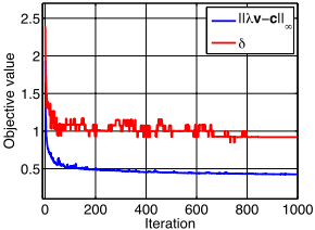
λ(ℓ) ‖ 1 1+e-Wxi - 1 1+e-Wxj ‖22 +‖xi - xj‖22 +y(ℓ) ij )2 , where λ(ℓ) denotes the value of λ in the ℓth iteration. We also use u(ℓ) ij and y(ℓ) ij to denote the entries in u(ℓ) and y(ℓ) that correspond to the pair (xi, xj) in the dataset X. We show in our experiments below that using the accelerated firstorder gradient descent algorithm [Nesterov, 2007] to solve this subproblem results in good convergence performance (see Figure 2).
- Optimize over u while holding the other variables fixed; this corresponds to solving the proximal problem of the ℓ∞- norm u(ℓ+1)←arg min u ‖u‖∞+ρ2 ‖u-λ(ℓ)v(ℓ+1)+c+y(ℓ) ‖22 .
We use the low-cost algorithm described in [Studer et al., 2014] to perform the proximal operator update.
- Optimize over λ while holding the other variables fixed; this corresponds to a positive least squares problem, where λ is updated as λ(ℓ+1)←arg min λ>0 1 2 ‖u(ℓ+1) - λv(ℓ+1) + c +
y(ℓ) ‖22 . We perform this update using the non-negative least squares algorithm.
- Update y via y(ℓ+1)←y(ℓ) +η(u(ℓ+1) -λ(ℓ+1)v(ℓ+1) +c), where the parameter η controls the dual update step size.
2.3 Accelerated RHash for Large-scale Datasets
The ADMM-based RHash algorithm is efficient for smallscale datasets (e.g., for secant sets of size |S(X)| < 5000 or so). However, the memory requirement of RHash is quadratic in |X |, which could be problematic for applications involving large numbers of data points and secants. In response, we develop an algorithm that approximately solves (P) while scaling very well to large-scale problems. The key idea comes from classical results in optimization theory related to column generation (CG) [Dantzig and Wolfe, 1960; Hegde et al., 2015].
The optimization (5) is an ℓ∞-norm minimization problem with an equality constraint on each secant. The KarushKuhn-Tucker (KKT) condition for this problem states that, if strong duality holds, then the optimal solution is entirely specified by a (typically very small) portion of the constraints. Intuitively, the secants corresponding to these constraints are the pairwise distances of kNNs that are harder to preserve in the low-dimensional Hamming space. We call this set of secants the active set. In order to solve (P), it suffices to find the active secants and solve the RHash optimization with that much smaller number of active constraints. To leverage the idea of the active set, we iteratively run RHash on a small subset of all of the secants that violate the distance preservation, as detailed below:
- Solve (P) with a small random subset S0 of all of the secants S(X) using RHash to obtain the initial estimates ̂W, ˆ δ, and ˆλ of the parameters. Identify the active set Sa. Fix λ = ˆλ for the rest of the algorithm.
- Randomly select a new subset Sv ⊂ S of secants that violate the distance preservation condition using the current estimates of ̂W, ˆ δ, and ˆλ. Then, form the augmented secant set Saug = Sa ∪ Sv.
- Solve (P) with the secants in the set Saug using the RHash algorithm.
We dub this approach RHash-CG. RHash-CG iterates over the above steps until no new violating secants are added to the active set. Since the algorithm searches over all secants for violations in each iteration, RHash-CG ensures that all of the constraints are satisfied when it terminates.
A key benefit of RHash-CG is that only the set of active secants (and not all of the secants) needs to be stored in memory. This leads to significant improvements in memory complexity over competing algorithms, since the size of the secant set grows quadratically with the number of data points and can quickly exceed the system memory capacity in largescale applications. The ℓ∞-norm distortion function enables RHash to leverage the simple CG approach in order to scale to larger datasets, another advantage of ℓ∞-norm for large-scale hashing.
2.4 RHash and NN Preservation Guarantee
Now that we have fully described the RHash algorithm, we develop a theory that bounds the probability of preserving all kNNs as a function of the ℓ∞-norm distortion measure δ minimized by RHash.
Inspired by the definition of relative contrast [He et al., 2012], we define a more generalized measure of data separability to preserve kNN that we call the k-order gap ∆k := d(x0, xk+1) - d(x0, xk), where x0 is a query point and xk and xk+1 are its kth and k + 1st NNs, respectively. We formally show that, if the data is sufficiently separable (∆k is large), then RHash preserves all kNNs with high probability under assumptions that are typical in the NN search literature [He et al., 2012] (see the appendix A for the proof).
Theorem 1. Assume that all of the data points are independently generated from a mixture of Gaussians distribution, i.e., xi ∼ ∑Pp=1 πpN(µp, Σp). Let x0 ∈ RN denote a query data point in the ambient space, and let the other data points xi be ordered such that d(x0, x1) < d(x0, x2) < . . . < d(x0, xQ). Let δ denote the ℓ∞-norm distortion parameter in RHash, and let c denote a positive constant. Then, if Ex[∆k] ≥ 2δ + ¨ 1c log Qk ϵ , then RHash preserves all kNNs of the query point x0 with probability at least 1 - ϵ.
3 Experiments
In this section, we validate the RHash and RHash-CG algorithms via experiments using a range of synthetic and realworld datasets, including three small-scale, three mediumscale, and one large-scale datasets. We use three metrics to compare RHash against ten state-of-the-art binary hashing algorithms, including binary reconstructive embedding (BRE) [Kulis and Darrell, 2009], spectral hashing (SH) [Weiss et al., 2009], anchor graph hashing (AGH) [Liu et al., 2011], multidimensional spectral hashing (MDSH) [Weiss et al., 2012], scalable graph hashing (SGH) [Jiang and Li, 2015], PCA hashing (PCAH), isotropic hashing (IsoHash) [Kong and Li, 2012], spherical Hamming distance hashing (SHD) [Heo et al., 2012], circulant binary embedding (CBE) [Yu et al., 2014], and locality-sensitive hashing (LSH) [Indyk and Motwani, 1998].
3.1 Performance Metrics and Datasets
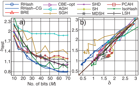
We compare the algorithms using the following three metrics: Maximum distortion δ = inf λ>0||λˆv - c||∞, where the vector ˆv contains the pairwise Hamming distances between the learned binary codes. This metric quantifies the distance preservation after projecting the training data in the ambient space into binary codes. We also define the maximum distortion for unseen test data δtest, which measures the distance preservation on a hold-out test dataset using the hash function learned from the training dataset.
Mean average precision (MAP) for NN preservation in the Hamming space. MAP is computed by first finding the set of kNNs for each query point in a hold-out test data set in the ambient space Lk and the corresponding set LkH in the Hamming space and then calculating the average precision AP = |Lk ∩ LkH|/k. We then report MAP by calculating the mean value of AP across all data points.
Kendall's τ ranking correlation coefficient. We first rank the set of kNNs for each data point by increasing distance in the ambient space as T (Lk ) and in the Hamming space as T (LkH). The Kendall τ correlation coefficient is a scalar τ ∈ [-1, 1] that measures the similarity between the two ranked sets T (Lk ) and T (LkH) The value of τ increases as the similarity between the two rankings increases and reaches the maximum value of τ = 1 when they are identical. We report the average value of τ achieved across all data points in the training dataset.
To compare the algorithms, we use the following standard datasets from computer vision: Random consists of independently drawn random vectors in R100 from a multivariate Gaussian distribution with zero mean and identity covariance matrix. Translating squares is a synthetic dataset consisting of 10×10 images that are translations of a 3×3 white square on a black background [Hegde et al., 2015]. MNIST is a collection of 60,000 28 × 28 greyscale images of handwritten digits [LeCun and Cortes, 1998]. Photo-Tourism is a corpus of approximately 300,000 image patches represented using scale-invariant feature transform (SIFT) features [Lowe, 2004] in R128 [Snavely et al., 2006]. LabelMe is a collection of over 20,000 images represented using GIST descriptors in R512 [Torralba et al., 2008]. Peekaboom is a collection of 60,000 images represented using GIST descriptors in R512 [Torralba et al., 2008]. Following the experimental approaches of the hashing literature [Kulis and Darrell, 2009; Norouzi and Fleet, 2011], we pre-process the data by subtracting the mean and then normalizing all points to lie on the unit sphere.
3.2 Small- andMedium-scale Experiments
We start by evaluating the performance of RHash and RHashCG using a subset of the first three datasets. Small-scale datasets enable comparisons between the asymptotic behaviors of the algorithms in preserving distances in a regime where number of bits is high enough (compared to the total number of NNs) to preserve a large portion of NN distances.
Experimental Setup. We randomly select Q = 100 data points from the Random, Translating squares, and MNIST datasets. We then apply the RHash, RHash-CG, and all of the baseline algorithms on each dataset for different target binary code word lengths M from 1 to 70 bits. We set the RHash and RHash-CG algorithm parameters to the common choice of ρ = 1 and η = 1.6. To generate a hash function of length M for LSH, we draw M random vectors from a Gaussian distribution with zero mean and an identity covariance matrix. We use the same random vectors to initialize RHash and the other baseline algorithms. In the NN preservation experiments, to demonstrate the direct advantage of minimizing ℓ∞-norm over ℓ2-norm, we followed the exact procedure described in BRE [Kulis and Darrell, 2009] to select the training secants, i.e., we apply the RHash algorithm on the lowest 5% of the pairwise distances (which are set to zero as in BRE) combined with the highest 2% of the pairwise distances.
We follow the continuation approach [Wen et al., 2010] to set the value of α. We start with a small value of α (e.g., α = 1), in order to avoid becoming stuck in bad local minima, and then gradually increase α as the algorithm proceeds. As the algorithm moves closer to convergence and has obtained a reasonably good estimate of the parameters W and λ, we set α = 10, which enforces a good approximation of the sign function (see Lem. 2 in the appendix A for an analysis of the accuracy of this approximation).
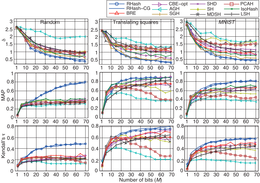
Results. The plots in the top row of Figure 3 illustrate the value of the distortion parameter δ as a function of the number of projections (bits) M. The performance of RHash and RHash-CG closely follow each other, indicating that RHash-CG is a good approximation to RHash. Both RHash and RHash-CG outperform the other baseline algorithms in terms of the distortion parameter δ. Among these baselines, LSH has the lowest distance preservation performance, which should be expected, since random projections are oblivious to the intrinsic geometry of the training dataset.
To achieve δ = 1, RHash(-CG) requires 60% fewer bits M than CBE and BRE. RHash(-CG) also achieves better distance preservation performance asymptotically, i.e., up to δ ≈ 0.5, given a sufficient number of bits (M ≥ 70), while for most of the other algorithms the performance plateaus after δ = 1. RHash's superior distance preservation performance extends well to unseen data. RHash achieves the lowest distortion on a test dataset δtest compared to the other hashing algorithms (Figure 4).
| MAP / Top-500 | Training time (s) | ||||
|---|---|---|---|---|---|
| Training size Q | 1k | 10k | 100k | 240k | 240k |
| Secant size |S(X)| | 100k | 10M | 1B | 5B | 5B |
| RHash-CG | 52.79 (±0.15) | 54.69 (±0.18) | 54.93 (±0.23) | 55.52 (±0.11) | 541.43 |
| CBE | 38.70 (±1.18) | 38.12 (±1.34) | 38.50 (±2.05) | 38.53 (±0.83) | 68.94 |
| SPH | 44.33 (±0.74) | 44.24 (±0.61) | 44.37 (±0.71) | 44.32 (±0.63) | 184.46 |
| SH | 40.12 (±0.00) | 39.37 (±0.00) | 38.79 (±0.00) | 38.26 (±0.00) | 3.05 |
| MDSH | 41.06 (±0.00) | 41.23 (±0.00) | 40.80 (±0.00) | 40.39 (±0.00) | 15.00 |
| AGH | 45.81 (±0.34) | 47.78 (± 0.38) | 47.69 (±0.41) | 47.38 (±0.32) | 4.49 |
| SGH | 51.32 (±0.07) | 51.33 (±0.20) | 51.01 (±0.23) | 50.66 (±0.76) | 5.89 |
| BRE | 48.33 (±0.65) | 50.67(±0.33) | - | - | 18685.51 |
| PCAH | 39.90 (±0.00) | 38.53 (±0.00) | 38.81 (±0.00) | 37.50 (±0.00) | 0.08 |
| IsoHash | 50.91 (±0.00) | 50.90 (±0.00) | 50.72 (±0.00) | 50.55 (±0.00) | 2.82 |
| LSH | 33.69 (±0.94) | 33.69 (±0.94) | 33.69 (±0.94) | 33.69 (±0.94) | 2.29 × 10⁻⁴ |
The plots in the middle and bottom row of Figure 3 show the average precision for retrieving training data and the Kendall's τ correlation coefficient respectively, as a function of the number of bits M. We see that RHash preserves a higher percentage of NNs compared to other baseline algorithms as M increases, with better average ranking among k = 10 NNs. We see that RHash preserves a higher percentage of NNs and achieves a better average ranking performance compared to other baseline algorithms.
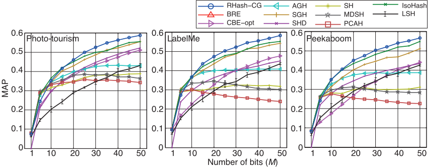
Next, we showcase the performance of RHash-CG on the three medium-scale, real-world datasets used in [Kulis and Darrell, 2009; Norouzi and Fleet, 2011], including Phototourism, LabelMe, and Peekaboom for the task of data retrieval. From each dataset we randomly select Q = 1000 training points, following the setup in BRE [Kulis and Darrell, 2009], and use them to train RHash-CG and the other baseline algorithms. We then randomly select a separate set of Q = 1000 data points and use it to test the performance of RHash-CG and other baseline algorithms in terms MAP with k = 50. Figure 5 illustrates the performance of RHash-CG on these datasets. RHash-CG outperforms all of the baseline algorithms by large margins in Hamming ranking performance in terms of MAP with top-50 NNs.
3.3 Large-scale Experiments
To demonstrate how RHash-CG scales to large-scale datasets, we use the full MNIST dataset with 60,000 training images and augment it with three rotated versions of each image (rotations of 90◦ , 180◦ , and 270◦ ) to create a larger dataset with Q = 240,000 data points. Next, we construct 4 training sets with 1,000, 10,000, 100,000, and 240,000 images out of this large set. We train all algorithms with M = 30 bits and compare their performance on a test set of 10,000 images. The results for all algorithms are given in Table 1; we tabulate their performance in terms of MAP for the top-500 NNs. 1 The performance of RHash-CG is significantly better than the baseline algorithms and, moreover, improves as the size of the training set grows.
4 Discussion
We have demonstrated that our worst-case, ℓ∞-normbased, Robust Hashing (RHash) algorithm is superior to a wide range of algorithms based on the more traditional average-case, ℓ2-norm. Despite its non-convexity and nonsmoothness, RHash admits an efficient optimization algorithm that converges to a high-performing local minimum. Moreover, RHash-CG, the accelerated version of RHash, provides significant memory advantages over existing algorithms; the memory requirement of RHash-CG is linear in the number of active secants rather than the total number of secants, a significant advantage over the existing reconstructive hashing methods which minimize the reconstruction error between the original distances in ambient space and the Hamming distances in embedded space. Our experiments with six datasets, three metrics, and ten algorithms have demonstrated the superiority of RHash over other state-of-the-art data-dependent hashing algorithms. Thus, our results provide a strong motivation for exploring ℓ∞-norm and other worstcase formulations for robust binary hashing.
A Proof of Theorem 1
Here, we prove Thm. 1 on the performance of RHash for k nearest neighbor (kNN) preservation.
We start with a result that bounds the error of the sigmoid approximation in RHash.
Lemma 2. Let x be a Gaussian random variable distributed as x ∼ N(µ, σ2 ). Define the distortion of the sigmoid approximation at x by |h(x) -σα(x)|. Then, the expected distortion is bounded by
1 BRE fails to execute on a standard desktop PC with 12 GB of RAM due to the size of the secant set.
where c is a positive constant. As α → ∞, the expected distortion → 0.
Proof. It is easy to see that the maximum distortion |h(x) - σα(x)| occurs at x = 0. Therefore, among different values of µ, µ = 0 gives the largest distortion, since the density of x peaks at x = 0. Therefore, we bound the distortion at setting µ = 0, which is an upper bound of the distortion when µ ̸= 0. By definition (1) above, h(x) can be written as
When x ∼N(0, σ2 ) and we set x0 = 1 √α , we can write
where c is a positive constant. In (6), we used the fact that σα(x) and h(x) are symmetric with respect to the point (0, 12 ). (7) follows from the properties of the sigmoid function; (8) follows from the Gaussian concentration inequality [Ledoux and Talagrand, 1991]; and (9) follows from the inequality 1/(1 + eαx0 ) ≤ e-αx0 . The fact that Ex[|h(x) -σα(x)|] → 0 as α → ∞ is obvious from the bound above.
Proof of Thm. 1
In order to prove Thm. 1, we need the following Lemma:
Lemma 3. Let x0, . . . , xN and ∆k be defined as in Thm. 1. Then, there exists a constant c such that P(∆k -Ex[∆k] < t) ≤ e-ct2 for t > 0.
Proof. Since the data points x0, xk and xk+1 are independently generated from a finite mixture of Gaussian distributions, the random variable of their concatenation y = [xT0 , xTk , xTk+1 ]T ∈ R3N is sub-Gaussian [Wainwright,
2009]. Then, we have
where we have used the triangular inequality in the second to last step, the Rayleigh-Ritz theorem, and the fact that the maximum singular value of the diagonal matrix above is 2. This means that ∆k(y) is a Lipschitz function of y. Thus, by Talagrand's inequality [Ledoux and Talagrand, 1991], we have that P(∆k - Ex[∆k] < -t) ≤ e-ct2 for some positive constant c and t > 0, since y is sub-Gaussian.
We are now ready to prove Thm. 1.
Proof. Let E denote the event that the set of top-k NNs is not preserved in the Hamming space. Then, we have E = ∪em,n, where em,n denotes the event that dH(x0, xm) > dH(x0, xn), with m ∈ {1, . . . , k} and n ∈ {k + 1, . . . , Q}. Then, using the union bound, we have
where we have used the fact that the most probable among all em,n events is the one corresponding to the order mismatch between the kth and k + 1st NN. Now, note that the RHash output δ satisfies maxi,j |dH(xi, xj) - d(xi, xj)| ≤ δ2 . Observe that ∆k = d(x0, xk+1)-d(x0, xk) ≥ 2δ is a sufficient condition for dH(x0, xk+1) ≥ dH(x0, xk), since
by the triangular inequality. This leads to
Combining all of the above with Lem. 3, the probability that the k NN is not preserved is bounded by
Now, by letting kQe-c(Ex[∆k]-2δ)2 ≤ ϵ, we have that the requirement for the top-k NNs to be exactly preserved with probability at least 1 - ϵ is Ex[∆k] ≥ 2δ + ¨ 1c log Qk ϵ .
2 Here we assume λ = 1 without loss of generality.
@inproceedings{ijcai2017p192,
  title     = {RHash: Robust Hashing via L_infinity-norm Distortion},
  author    = {Aghazadeh, Amirali and Lan, Andrew and Shrivastava, Anshumali and Baraniuk, Richard},
  booktitle = {Proceedings of the Twenty-Sixth International Joint Conference on
               Artificial Intelligence, {IJCAI-17}},
  publisher = {International Joint Conferences on Artificial Intelligence Organization},
  editor    = {Carles Sierra, IIIA-CSIC},
  pages     = {1386--1394},
  year      = {2017},
  month     = {8},
  note      = {Main track},
  doi       = {10.24963/ijcai.2017/192},
  url       = {https://doi.org/10.24963/ijcai.2017/192},
}
TY - CPAPER TI - RHash: Robust Hashing via L_infinity-norm Distortion AU - Aghazadeh, Amirali AU - Lan, Andrew AU - Shrivastava, Anshumali AU - Baraniuk, Richard T2 - Proceedings of the Twenty-Sixth International Joint Conference on Artificial Intelligence, IJCAI-17 PB - International Joint Conferences on Artificial Intelligence Organization PY - 2017 SP - 1386 EP - 1394 DO - 10.24963/ijcai.2017/192 UR - https://doi.org/10.24963/ijcai.2017/192 ER -Copied
Machine-readable versions of this paper, for tools and AI agents:





