
Self-weighted Multiview Clustering with Multiple Graphs
Proceedings of the Twenty-Sixth International Joint Conference on Artificial Intelligence. Main track. Pages 2564-2570.
https://doi.org/10.24963/ijcai.2017/357
Keywords
- Machine Learning: Unsupervised Learning
- Machine Learning: Data Mining
Abstract
In multiview learning, it is essential to assign a reasonable weight to each view according to its importance. Thus, for multiview clustering task, a wise and elegant method should achieve clustering multiview data while learning the view weights. In this paper, we address this problem by exploring a Laplacian rank constrained graph, which can be approximately as the centroid of the built graph for each view with different confidences. We start our work with a natural thought that the weights can be learned by introducing a hyperparameter. By analyzing the weakness of it, we further propose a new multiview clustering method which is totally self-weighted. Furthermore, once the target graph is obtained in our models, we can directly assign the cluster label to each data point and do not need any postprocessing such as $K$-means in standard spectral clustering. Evaluations on two synthetic datasets prove the effectiveness of our methods. Compared with several representative graph-based multiview clustering approaches on four real-world datasets, experimental results demonstrate that the proposed methods achieve the better performances and our new clustering method is more practical to use.
- [Asuncion and Newman, 2007] Arthur Asuncion and David Newman. Uci machine learning repository, 2007.
- [Blum and Mitchell, 1998] Avrim Blum and Tom Mitchell. Combining labeled and unlabeled data with co-training. In Proceedings of the eleventh annual conference on Compu- tational learning theory, pages 92-100. ACM, 1998.
- [Cai et al., 2005] Deng Cai, Xiaofei He, and Jiawei Han. Document clustering using locality preserving indexing. Knowledge and Data Engineering, IEEE Transactions on, 17(12):1624-1637, 2005.
- [Cai et al., 2011] Xiao Cai, Feiping Nie, Heng Huang, and Farhad Kamangar. Heterogeneous image feature integra- tion via multi-modal spectral clustering. In Computer Vi- sion and Pattern Recognition (CVPR), 2011 IEEE Confer- ence on, pages 1977-1984. IEEE, 2011.
- [Chen and Dy, 2016] Junxiang Chen and Jennifer Dy. A gen- erative block-diagonal model for clustering. In Proceed- ings of the Thirty-Second Conference on Uncertainty in Artificial Intelligence, UAI 2016, June 25-29, 2016, New York City, NY, USA, 2016.
- [Cheng and Zhao, 2009] Yong Cheng and Ruilian Zhao. Multiview spectral clustering via ensemble. In Granu- lar Computing, 2009, GRC'09. IEEE International Con- ference on, pages 101-106. IEEE, 2009.
- [Chung, 1997] Fan RK Chung. Spectral graph theory, vol- ume 92. American Mathematical Soc., 1997.
- [Daubechies et al., 2010] Ingrid Daubechies, Ronald De- Vore, Massimo Fornasier, and C Sinan Güntürk. Iterative- ly reweighted least squares minimization for sparse recov- ery. Communications on Pure and Applied Mathematics, 63(1):1-38, 2010.
- [Duchi et al., 2008] John Duchi, Shai Shalev-Shwartz, Y- oram Singer, and Tushar Chandra. Efficient projections onto the l 1-ball for learning in high dimensions. In Pro- ceedings of the 25th international conference on Machine learning, pages 272-279. ACM, 2008.
- [Fan, 1950] Ky Fan. On a theorem of weyl concerning eigen- values of linear transformations ii. Proceedings of the Na- tional Academy of Sciences, 36(1):31-35, 1950.
- [Fei-Fei et al., 2007] Li Fei-Fei, Rob Fergus, and Pietro Per- ona. Learning generative visual models from few train- ing examples: An incremental bayesian approach tested on 101 object categories. Computer Vision and Image Un- derstanding, 106(1):59-70, 2007.
- [Feng et al., 2014] Jiashi Feng, Zhouchen Lin, Huan Xu, and Shuicheng Yan. Robust subspace segmentation with block-diagonal prior. In Proceedings of the IEEE Confer- ence on Computer Vision and Pattern Recognition, pages 3818-3825, 2014.
- [Kumar and Daumé, 2011] Abhishek Kumar and Hal Daumé. A co-training approach for multi-view spectral clustering. In Proceedings of the 28th International Conference on Machine Learning (ICML-11), pages 393-400, 2011.
- [Kumar et al., 2011] Abhishek Kumar, Piyush Rai, and Hal Daumeé. Co-regularized multi-view spectral clustering. In Advances in Neural Information Processing Systems, pages 1413-1421, 2011.
- [Li et al., 2015] Yeqing Li, Feiping Nie, Heng Huang, and Junzhou Huang. Large-scale multi-view spectral cluster- ing via bipartite graph. In AAAI, pages 2750-2756, 2015.
- [Mohar et al., 1991] Bojan Mohar, Y Alavi, G Chartrand, and OR Oellermann. The laplacian spectrum of graph- s. Graph theory, combinatorics, and applications, 2(871- 898):12, 1991.
- [Nie et al., 2010] Feiping Nie, Heng Huang, Xiao Cai, and Chris H Ding. Efficient and robust feature selection via joint ℓ 2,1 -norms minimization. In Advances in neural in- formation processing systems, pages 1813-1821, 2010.
- [Nie et al., 2014a] Feiping Nie, Xiaoqian Wang, and Heng Huang. Clustering and projected clustering with adaptive neighbors. In The 20th ACM SIGKDD International Con- ference on Knowledge Discovery and Data Mining, KDD, pages 977-986, 2014.
- [Nie et al., 2014b] Feiping Nie, Jianjun Yuan, and Heng Huang. Optimal mean robust principal component analy- sis. In Proceedings of the 31st International Conference on Machine Learning (ICML-14), pages 1062-1070, 2014.
- [Nie et al., 2016a] Feiping Nie, Jing Li, and Xuelong Li. Parameter-free auto-weighted multiple graph learning: A framework for multiview clustering and semi-supervised classification. In Proceedings of the Twenty-Fifth Inter- national Joint Conference on Artificial Intelligence, pages 1881-1887, 2016.
- [Nie et al., 2016b] Feiping Nie, Xiaoqian Wang, Michael I Jordan, and Heng Huang. The constrained laplacian rank algorithm for graph-based clustering. 2016.
- [Tang et al., 2009] Wei Tang, Zhengdong Lu, and Inderjit S Dhillon. Clustering with multiple graphs. In Data Mining, 2009. ICDM'09. Ninth IEEE International Conference on, pages 1016-1021. IEEE, 2009.
- [Winn and Jojic, 2005] John Winn and Nebojsa Jojic. Locus: Learning object classes with unsupervised segmentation. In Computer Vision. Tenth IEEE International Conference on, volume 1, pages 756-763. IEEE, 2005.
- [Xia et al., 2014] Rongkai Xia, Yan Pan, Lei Du, and Jian Yin. Robust multi-view spectral clustering via low-rank and sparse decomposition. In AAAI, pages 2149-2155, 2014.
- [Xie and Sun, 2013] Xijiong Xie and Shiliang Sun. Multi- view clustering ensembles. In Machine Learning and Cybernetics (ICMLC), 2013 International Conference on, volume 1, pages 51-56. IEEE, 2013.
- [Zelnik-Manor and Perona, 2005] Lihi Zelnik-Manor and Pietro Perona. Self-tuning spectral clustering. 2005.
References were extracted automatically from the PDF and may contain errors.
Full text extracted automatically from the PDF; figures, tables and equations may differ. The PDF is the version of record.
1 Introduction
Many computer vision objects, such as image and video, involve instances represented with multiple views. It is essential to study how to efficiently cluster such kind of data. Suppose we use a graph to capture entities and their relation in each view, we will naturally obtain multiple graphs. Therefore, from this perspective, graph-based multiview clustering can be transformed into a multiple graph learning problem.
Prior to the multiple graph learning method, a direct way to handle multiview data is to concatenate all the features into a new one and then utilize it to construct a single graph. However, this seemingly simple method neglects the relation among all the views and doesn't make sense theoretically. Recently, in pratice many works would prefer to construct a graph for each view and then jointly utilize them to learn a unified one. Inspired by co-training [Blum and Mitchell, 1998], which is widely used in multiview semisupervised learning, [Kumar and Daum´e, 2011] searched for the clusters that agree across all the views. Later, to minimize the disagreement between every pair of views, [Kumar et al., 2011] applied the co-regularization technique to spectral clustering model and reformulated multiview clustering as a jointly maximization problem. Similarly, [Cai et al., 2011] designed a graph-based multiview spectral learning model to integrate heterogenous image features. These methods extend pairwise concept to multiple views condition and look for the most consistent representation. Following a more comprehensive thought is that each individual view may contain specific information as well as common information, [Tang et al., 2009] presented the linked matrix factorization model to extract the structure information shared by all the graphs.
Almost every aforementioned method works on the assumption that all the views are reliable. However, in realworld clustering problems, the views of data are inherently strong or weak, and meanwhile some may have been corrupted by noises. This means the final results will be degraded if we fail to distinguish different views. [Xia et al., 2014] addressed this problem by separating noise from each graph and learned a shared low-rank transition probability matrix, which will be the input to the standard Markov chain method for clustering. [Kumar et al., 2011; Cheng and Zhao, 2009] proposed to roughly compute the weights by combining with the prior knowledge. This kind of approaches are manually intervening or shallow. In view of this point, some other methods [Li et al., 2015; Xie and Sun, 2013] looked for a new weight learning strategy which has been widely used in multiview learning. It explicitly defines the view weights in the objective and then learns them as variables, which is parallel with the thought of our first method. Nevertheless, this so-called adaptive or automatical weight learning strategy has to resort to an additional hyperparameter (For simplicity, we replace with γ when referring this parameter in the following text), which is usually difficult to set in a specific task.
The first motivation of this work is: it is very common that graph-based clustering methods appear in the context of spectral learning, such as [Kumar and Daum´e, 2011; Kumar et al., 2011; Cai et al., 2011; Tang et al., 2009; Xia et al., 2014; Cheng and Zhao, 2009; Li et al., 2015; Xie and Sun, 2013]. This means that in the last step of these methods, it often needs to apply a simple clustering method such as K-means to the learned indicator matrix. However, the uncertainty of this postprocessing operation will increase the instability of the original performance. We avert this trouble by extending an existing single graph learning approach [Nie et al., 2016b] to multiview domain. Inspired by the recent works, we propose the Parameter-weighted Multiview Clustering (PwMC) method to weightedly combine each single graph learning model. The second motivation is that, as many previous works, PwMC involves an undesired parameter γ. There are two reasons to argue. 1) In context of unsupervised learning where no instance is labeled, γ can not be obtained by traditional supervised hyperparameter tuning techniques, such as cross validation. 2) It is observed that the final experimental performance is sensitive to γ and the optimum of γ varies on different datasets (see Experiments part of Section 3.3), which causes PwMC (and the related multiview clustering methods with the similar weight learning strategy) not practical to use. Thus, to remove γ while without loss of too much precision, we further propose a new Self-weighted Multiview Clustering (SwMC) method. These two motivations are exactly corresponding to our contributions of this paper. The toy examples and experiments on real-world datasets demonstrate the the effectiveness of our proposed methods.
Notation. Throughout the paper, all the matrices are written as uppercase. For a matrix M, the i-th row and ij-th element of M are denoted as mi and mij separately. The trace of M is denoted as Tr(M). The v-th view representation of M is written as M (v) . The Frobenius norm of matrix M is denoted by ‖M‖F . In particular, we use 1n to denote a n dimensional column vector where each element is 1.
2 The Proposed Framework
2.1 Graph-based Clustering Revisit
Suppose we have n samples and they can be partitioned into c clusters, graph-based clustering methods firstly construct a Similarity Matrix (SM, and we will not differ SM and graph in this paper) to represent the affinities of all the samples. Many early works have studied how to design a SM with high quality, such as [Zelnik-Manor and Perona, 2005; Cai et al., 2005]. These well-designed SMs will be the inputs of graph-based clustering methods, e.g., spectral clustering. However, an ideal SM S ∈ Rn×n is supposed to exactly have c connected components, by which way, S can be directly used for the clustering task. Recently, [Nie et al., 2014a; Feng et al., 2014; Chen and Dy, 2016; Nie et al., 2016b] have leveraged this property in different ways. We briefly introduce the Constrained Laplacian Rank (CLR) method [Nie et al., 2016b] therein, which is easier to understand and will be the base of our proposed framework. Given an arbitrary input SM A ∈ Rn×n , the target SM can be learned by minimizing the following problemmin
where S is nonnegative, whose each row sums up to 1, and C represents the set of n by n square matrices with c connected components. According to the graph theory in [Mohar et al., 1991; Chung, 1997], the connectivity constraint can be replaced with a rank constraint, and thus we have
where rank(LS) means the rank of LS. The Laplacian matrix LS = DS - (ST +S)/2, where the degree matrix DS ∈ Rn×n is defined as a diagonal matrix whose i-th diagonal element is ∑j (sij + sji)/2. In this way, the target SM can be solved and we directly use it for clustering.
2.2 Parameter-weightedMultiviewClustering (PwMC)
CLR is a single view graph-based clustering method. In this paper, we introduce this technique into multiview clustering domain. For multiview data, let m be the number of views and A(1) ,A(2) , ...,A(m) be the corresponding input SMs, where A(v) ∈ Rn×n (1 ≤ v ≤ m). Thus, our goal becomes to find out the target SM S which is constrained as in Eq. (2) but can approximate each original input SMA(v) . An intuitive way to address this problem is to simply calculate an average SM A = 1m m∑ A(v) and input it into CLR. Actu-
ally, this thought is equivalent to assigning the equal weight to each graph. In practice, we need to employ a group of meaningful weights to measure the importance of each view. In other words, the target SM S is supposed to approximate every input SM with different confidences. This idea can be naturally modeled by minimizing the linear combination of the reconstruction error ∥∥S -A(v)∥∥2F for each view. Thus, the formulated objective can be written as
where α = [α(1) , α(2) , ..., α(m) ]T and γ > 0. The second term in problem (3) is used to smoothen the weight distribution. Straightforward, without this regularization term (or γ → 0), the trivial solution will be obtained, i.e., the weight of best view will be assigned to 1 and other weights will be 0s. On the contrary, when γ →∞, the equal weights will be obtained. Since the weights severely depend on the parameter γ, we name this method as Parameter-weighted Multiview Clustering (PwMC). The detailed procedure of optimize the problem (3) is presented in Section 2.4.
2.3 Self-weightedMultiviewClustering (SwMC)
Although problem (3) provides a feasible scheme to fuse multiple graphs on the model level, it involves the undesired parameter γ, which is confirmed to be dataset-related by our experiments. To remove the parameter γ in problem (3), we propose a self-weighted multiview clustering method. It sounds unreasonable that the suitable weights could be generated out of thin air. But in this part, we present a new formulation that actually induces a self-conducted weight learning. The proposed objective is
This equation looks pretty simplified and compact, but no weight factor is explicitly defined therein. We consider it as a normal issue and firstly write its Lagrange function
where Λ is the Lagrange multiplier, G (Λ, S) serves as a proxy for the constraints to S. Taking the derivative of Eq. (5) w.r.t S and setting the derivative to zero, we have
where w(v) is given as the following form 1
Obviously, from Eq. (7) we know that w(v) is dependent on S, which means the two factors of the first term in Eq. (6) are coupled with each other. But if we set w(v) stationary, Eq. (6) can be considered as the solution to the following problem
which is simpler to be solved. And then, the calculated S from problem (8) can be further used to update w(v) by Eq. (7). This inspires us to solve the original problem (4) by alternately optimizing S and w(v) iteratively. We summarize this process into Algorithm 1. Moreover, if this alternating optimization strategy converges (it will be proved later), from Eq. (6) we know that the finally learned S will converge to the KKT condition of the problem (4).
Algorithm 1 The algorithm of Self-weighted Multiview Clustering (SwMC) in Eq. (4)
Input: SMs for m views {A(1) , A(2) , ..., A(m)} and A(v) ∈
Rn×n , number of clusters c.
Initialize the weight for each view (e.g., α(v) = 1m ).
repeat
- Calculate S by solving the problem (8).
- Update α(v) by using Eq. (7).
until converge Output: S ∈ Rn×n with exactly c connected components So far, we have presented the general process to solve the problem (4). But what is the relation between it and our selfweighted multiview learning? Inspecting Eq. (8), when the optimization process converges, its form can be described as the linear combination of reconstruction errors of different views if we view the w(v) as the weight factor, which is exactly what we want to learn. Since Eq. (8) is derived from solving the problem (4), it is a totally self-weighted process. Furthermore, if view v is good, then ∥∥S -A(v)∥∥F should be small, and thus the learnt w(v) for view v is large according to Eq. (7). Accordingly, a weak view will be assigned a small weight. This indicates that our self-weighted learning model is meaningful. In fact, the above process of solving problem (4) can be seen as a special case of the Iteratively Re-weighted (IR) technique [Nie et al., 2010; Daubechies et al., 2010; Nie et al., 2014b]. In this perspective, the effectiveness of this method will reflect the practical significance of the weight formula in IR.
1 To avoid dividing by zero, in practice we use the following formula w(v) = 1/(2√‖S -A(v) ‖2F + δ), where δ is some very small value, like 0.0001.
2.4 Optimization
Optimization of PwMC
Once given a proper value of parameter γ, we can adopt the alternating iterative strategy to optimize the problem (3).
When α is fixed, we need to solve the following subproblem
Let σi (LS) denote the i-th smallest eigenvalue of LS. σi (LS) ≥ 0 since LS is positive semi-definite. Given a large enough λ2 , the rank constraint in Eq. (9) can be eliminated and the problem (9) is equivalent to the following form:
When λ is large enough, note that σi (LS) ≥ 0 for each i, thus the optimal solution S to the problem (10) will make the second term c∑ i=1 σi (LS) equal to zero and the constraint rank(LS) = n - c will be satisfied. In addition, according to Ky Fan's Theory [Fan, 1950], we have the following equation:
Thus, combining with Eq. (11), the problem (10) is further equivalent to the following problem:
2 Unlike the regular hyperparameter, this introduced λ will not influence the final experimental performance. In our method, following the CLR method, we determine the value of λ in a heuristic way to accelerate the procedure.
We solve this problem by optimizing variables F and S iteratively as follows.
- Solving F When S is fixed, the problem (12) becomes
It is known that the optimal solution of F is formed by the c eigenvectors of LS corresponding to the c smallest eigenvalues.
ii. Solving S When F is fixed, the problem (12) becomes
Since the problem (14) is independent for different i, we can solve the following problem separately for each i:
For simplicity, we denote vij = ‖fi - fj‖22 and vi as a vector with j-th element equal to vij (and similarly for si and ai), the problem (15) can be written in vector form as
This problem can be solved by an efficient iterative algorithm proposed in [Duchi et al., 2008]. To accelerate the computing, we can choose to update t (One can set t as a const, like 10) neighbors of i-th data. Thus, S is totally sparse and can be rapidly calculated.
When S is fixed, the problem (3) is reduced to minimization to the following problem
where e(v) = ∥∥S -A(v)∥∥2F . It is easy to rewrite the problem (17) into the following form
which is identical with the problem (16). Now, we summarize the solving process of problem (3) in Algorithm 2.
Optimization of SwMC
According to Algorithm 1, solving SwMC mainly contains two alternative steps, in which updating by Eq. (7) is quite simple while the subproblem (8) needs to be further calculated. Seeing that the only difference between problems (8) and (9) is whether weights sums up to 1, thus we can solve the subproblem (8) with the same way.
2.5 Converge Analysis
According to the alternating optimization steps described in Algorithm 2, since we can find the optimal solution of each Algorithm 2 The algorithm of Parameter-weighted Multiview Clustering (PwMC) in Eq. (3)
Input: SMs for m views {A(1) , A(2) , ..., A(m)} and A(v) ∈ Rn×n , number of clusters c, parameter γ.
Initialize the weight for each view (e.g., α(v) = 1m ). Let A = m∑ v=1 α(v)A(v) , and compute F ∈ Rn×c , which is
formed by the c eigenvectors of LA = DA - AT +A 2 corresponding to the c smallest eigenvalues.
repeat repeat
i. For each i, update the i-th row of S by solving the problem (16).
ii. Update F, which is formed by the c eigenvectors of LS = DS - ST +S 2 corresponding to the c smallest eigenvalues.
until converge
Update the weight α(v) by solving the problem (18). until converge
Output: S ∈ Rn×n with exactly c connected components.
subproblem, obviously Algorithm 2 will converge. Now, we focus on proving the convergence of Algorithm 1.
Lemma 1 [Nie et al., 2010] For any positive number u and v, the following inequality holds:
Theorem 1 In each iteration of Algorithm 1, the updated target SM S will monotonically decrease the objective of problem (4), which generally makes the solution converge to the local optimum of the problem (4) .
Proof: Let ˜ S denote the updated S in each iteration. According to the first step of loop in Algorithm 1, we have
Combining with w(v) = 1/(2∥∥S - A(v)∥∥F ), we can derive
According to Lemma 1, we have
Summing Eq. (21) and Eq. (22) in the two sides, we arrive at
| View | MSRCv1 | Cal-7(20) | Digits |
|---|---|---|---|
| 1 2 3 4 5 | CM(24) HOG(576) GIST(512) LBP(256) | Gabor(48) | FOU(76) |
| WM(40) | FAC(216) | ||
| CENT(254) | KAR(64) | ||
| HOG(1984) | PIX(240) | ||
| CENT(254) | GIST(512) | ZER(47) | |
| 6 | - | LBP(928) | MOR(6) |
| # Size | 210 | 1474(2386) | 2000 |
| # Classes | 7 | 7(20) | 10 |
Thus, the iterative optimization will monotonically decease the objective of the problem (4) in each iteration until it converges. When the convergence reaches, the equality in Eq. (22) holds, thus ˜ S will satisfy Eq. (6), the KKT condition of problem (4). Therefore, in most cases, the Algorithm 1 will at least converge to a local optimal solution of problem (4).
3 Experiments
In this paper, we follow CLR method to construct a graph for each view as the initialized input graph A(v) . Different from some regular kernel-based methods [Zelnik-Manor and Perona, 2005; Cai et al., 2005], this graph construction approach only needs to set one parameter k which represents the number neighbors. For all the compared methods, we validate their performances by fixing k as 10. Another advantage is that this approach naturally obtains the neat normalized graph for each view. It is a hard-to-get property, and many previous graph construction methods have to normalize multiview data before utilization. The standard clustering Purity and Normalized Mutual Information (NMI) metrics are used to measure the clustering performance in our experiments.
3.1 Toy Example
In this part, we conduct two toy experiments to verify the effectiveness of the proposed algorithms.
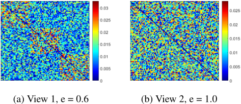
Toy 1 dataset. We design a two-view synthetic dataset where each view is a 90×90 matrix with three 30×30 block matrices diagonally arranged. Without loss of generality, the data within each block denotes the affinity of two corresponding points in one cluster, while the data outside all blocks denotes noise. Each element in all blocks is randomly generated in the range of 0 and 1, while the noise data is randomly generated in the range of 0 and e, where e is set as 0.6 in the 1st matrix, and 1.0 in the 2nd matrix. Then they are normalized to be that the sum of each row is 1. The original input graphs are shown in Figure 1.
We have verified that CLR can directly recover the desired block diagonal matrix from view 1 but fails on view 2. Given some small value to the parameter γ, the learned weights of PwMC are close to 1/0 , which means in such a situation PwMC achieves the best performance (For the space limitation, we won't present all the learned clean block diagonal matrix.) by selecting the best view. For SwMC, it also learns the clean block diagonal matrix but with the normalized weights
0.63/0.37. Seeing that the elements within diagonally blocks always contributes to clustering, it indicates that SwMC arrives at the optimal solution in a different style.
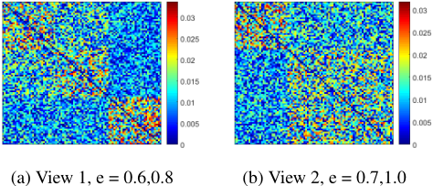
Toy 2 dataset. This synthetic dataset has the same scale with Toy 1 but with the different noise settings. The initial noise in view 1 and 2 is set as e = 0.6 and e = 0.7 respectively. By increasing the noise between the first and second block data to e = 0.8, we obtain the input matrix for view 1. Similarly, in view 2, we increase the noise between the second and third block data to e = 1.0. They are are normalized and then shown as Figure 2.
By performing CLR on each individual graph, their clustering performance are : Purity of view 1 and 2 are 0.66/0.63, NMI of view 1 and 2 are 0.58/0.58. The proposed methods can still integrate these two complementary graphs and recover the clean block diagonal matrix. The learned weights of both proposed methods are around 0.53/0.47. Noting that view 1 contains less noise than view 2, for SwMC method, according to Eq. (7), we find this phenomenon agrees with our prior inference in Section 2.3.
3.2 Performance Evaluation
Following [Li et al., 2015], we evaluate the performance of the compared methods on three multi-view datasets, MSRCv1 [Winn and Jojic, 2005], Caltech101 [Fei-Fei et al., 2007] (we use two regular subsets Caltech101-7 and Caltech10120), Handwritten numerals (Digits) [Asuncion and Newman, 2007], which are briefly summarized in Table 1.
We compare the proposed PwMC and SwMC with following methods: Co-regularized spectral clustering [Kumar et al., 2011] (Co-reg), Multi-View Spectral Clustering [Cai et al., 2011] (MVSC), Robust Multi-view Spectral Clustering [Xia et al., 2014] (RMSC). For each compared method, the parameter is allowed to be tuned as optimum (never forget that the proposed SwMC has no parameter to tune except for the prefixed cluster number k). Meanwhile, to reduce the influence of the postprocessing to the learned indicator matrix, for all the methods involving K-means, we repeat them for 50 times and report the averaged result. As for our methods, we only run once. We mark the top two results in bold face.
| MSRCv1 | Caltech101-7 | Caltech101-20 | Digits | |||||
|---|---|---|---|---|---|---|---|---|
| Purity | NMI | Purity | NMI | Purity | NMI | Purity | NMI | |
| CLRbest | 0.6143 | 0.6005 | 0.8437 | 0.5221 | 0.6102 | 0.3761 | 0.8720 | 0.8759 |
| Co-reg | 0.6243 | 0.5924 | 0.6669 | 0.3227 | 0.5624 | 0.4879 | 0.8243 | 0.8068 |
| MVSC | 0.7286 | 0.6152 | 0.8453 | 0.5972 | 0.7045 | 0.5025 | 0.8610 | 0.8532 |
| RMSC | 0.7295 | 0.6138 | 0.8047 | 0.4788 | 0.7083 | 0.4903 | 0.7794 | 0.7349 |
| PwMC | 0.8857 | 0.8062 | 0.8548 | 0.5713 | 0.7137 | 0.5121 | 0.8800 | 0.8925 |
| SwMC | 0.8667 | 0.7835 | 0.8548 | 0.5423 | 0.7137 | 0.5121 | 0.8815 | 0.8934 |
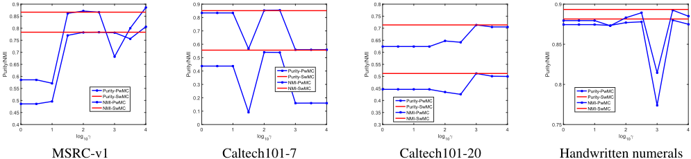
Table 2 shows the clustering Purity and NMI of all the methods on four datasets respectively. The best result of CLR is set as the baseline in this experiment. In general, the proposed methods in most cases achieve the top two performances among the compared state-of-the-art multiview clustering methods. Meanwhile, we find that Co-reg achieves the unsatisfactory results, which is due to the fact that we have no prior knowledge to support the weight assignment and thus weight learning is not conducted in this scheme. For RMSC, it usually obtains the decent results but sometimes fails, especially on digit recognition tasks. As we mention before, RMSC differs diverse views by peeling the assumed noise (error) from each built graph and learning a clean and unified one. Thus, a convincing explanation for that failure case is that RMSC cannot handle the views in which some are naturally dominant while others are pretty weak. MVSC searches a linear combination of different view's graphs, whose performance is slightly inferior to our graph structure based multiview clustering method.
3.3 Parameter-freeWeight Learning
Figure 3 exhibits the clustering performance of the proposed SwMC comparing with PwMC on different datasets. Typically, γ in PwMC is searched in logarithm form (log10γ from 0 to 4 with step size 0.5). Although PwMC and SwMC are influenced by the different initializations, we start then with the equal weights in this experiment.
According to Figure 3, except for Digits, PwMC achieves better (or at least equal) performance than SwMC at some specific γ. Theoretically, a specific γ corresponds to a weight distribution, which means the optimal weight combination will be obtained if one can search all the possible γs. However, it is observed that the performance of PwMC varies dramatically when γ changes, which makes that attempting to apply a fixed γ throughout all the applications is not practical. Therefore, the proposed method SwMC is preferred. This new multiview clustering method does not depend on an additional parameter to learn the weights and without much precision loss, is interesting and can be acceptable.
4 Conclusion
In this paper, to recover the block diagonal matrix from multiple original input graphs, we firstly propose Parameterweighted Multiview Clustering (PwMC) method. By analyzing its weaknesses, we further propose a new weight leaning strategy in multiview clustering, named as Self-weighted Multiview Clustering (SwMC). The proposed methods are verified on two toy datasets and four benchmark datasets. Experimental results demonstrate the effectiveness of our methods. Especially, we note that SwMC achieves the close performance with PwMC but is practical to use. In future work, like [Nie et al., 2016a], we will consider extending this framework to semi-supervised context.
@inproceedings{ijcai2017p357,
  title     = {Self-weighted Multiview Clustering with Multiple Graphs},
  author    = {Nie, Feiping and Li, Jing and Li, Xuelong},
  booktitle = {Proceedings of the Twenty-Sixth International Joint Conference on
               Artificial Intelligence, {IJCAI-17}},
  publisher = {International Joint Conferences on Artificial Intelligence Organization},
  editor    = {Carles Sierra, IIIA-CSIC},
  pages     = {2564--2570},
  year      = {2017},
  month     = {8},
  note      = {Main track},
  doi       = {10.24963/ijcai.2017/357},
  url       = {https://doi.org/10.24963/ijcai.2017/357},
}
TY - CPAPER TI - Self-weighted Multiview Clustering with Multiple Graphs AU - Nie, Feiping AU - Li, Jing AU - Li, Xuelong T2 - Proceedings of the Twenty-Sixth International Joint Conference on Artificial Intelligence, IJCAI-17 PB - International Joint Conferences on Artificial Intelligence Organization PY - 2017 SP - 2564 EP - 2570 DO - 10.24963/ijcai.2017/357 UR - https://doi.org/10.24963/ijcai.2017/357 ER -Copied
Machine-readable versions of this paper, for tools and AI agents:





