
Approximating Discrete Probability Distribution of Image Emotions by Multi-Modal Features Fusion
Proceedings of the Twenty-Sixth International Joint Conference on Artificial Intelligence. Main track. Pages 4669-4675.
https://doi.org/10.24963/ijcai.2017/651
Keywords
- Uncertainty in AI: Approximate Probabilistic Inference
- Robotics and Vision: Vision and Perception
Abstract
Existing works on image emotion recognition mainly assigned the dominant emotion category or average dimension values to an image based on the assumption that viewers can reach a consensus on the emotion of images. However, the image emotions perceived by viewers are subjective by nature and highly related to the personal and situational factors. On the other hand, image emotions can be conveyed by different features, such as semantics and aesthetics. In this paper, we propose a novel machine learning approach that formulates the categorical image emotions as a discrete probability distribution (DPD). To associate emotions with the extracted visual features, we present a weighted multi-modal shared sparse leaning to learn the combination coefficients, with which the DPD of an unseen image can be predicted by linearly integrating the DPDs of the training images. The representation abilities of different modalities are jointly explored and the optimal weight of each modality is automatically learned. Extensive experiments on three datasets verify the superiority of the proposed method, as compared to the state-of-the-art.
- [Alameda-Pineda et al., 2016] Xavier Alameda-Pineda, Elisa Ric- ci, Yan Yan, and Nicu Sebe. Recognizing emotions from abstract paintings using non-linear matrix completion. In CVPR, pages 5240-5248, 2016.
- [Borth et al., 2013] Damian Borth, Rongrong Ji, Tao Chen, Thomas Breuel, and Shih-Fu Chang. Large-scale visual sentiment ontol- ogy and detectors using adjective noun pairs. In ACM MM, pages 223-232, 2013.
- [Carney et al., 2005] Michael Carney, Pádraig Cunningham, Jim Dowling, and Ciaran Lee. Predicting probability distributions for surf height using an ensemble of mixture density networks. In ICML, pages 113-120, 2005.
- [Chartrand and Yin, 2008] Rick Chartrand and Wotao Yin. Itera- tively reweighted algorithms for compressive sensing. In ICAS- SP, pages 3869-3872, 2008.
- [Chen et al., 2014] Tao Chen, Felix X Yu, Jiawei Chen, Yin Cui, Yan-Ying Chen, and Shih-Fu Chang. Object-based visual senti- ment concept analysis and application. In ACM MM, pages 367- 376, 2014.
- [Ding et al., 2016] Guiguang Ding, Yuchen Guo, Jile Zhou, and Yue Gao. Large-scale cross-modality search via collective matrix factorization hashing. IEEE Transactions on Image Processing, 25(11):5427-5440, 2016.
- [Ekman, 1992] Paul Ekman. An argument for basic emotions. Cog- nition & Emotion, 6(3-4):169-200, 1992.
- [James and Dasarathy, 2014] Alex Pappachen James and Belur V Dasarathy. Medical image fusion: A survey of the state of the art. Information Fusion, 19:4-19, 2014.
- [Jia et al., 2014] Yangqing Jia, Evan Shelhamer, Jeff Donahue, Sergey Karayev, Jonathan Long, Ross Girshick, Sergio Guadar- rama, and Trevor Darrell. Caffe: Convolutional architecture for fast feature embedding. In ACM MM, pages 675-678, 2014.
- [Joshi et al., 2011] Dhiraj Joshi, Ritendra Datta, Elena Fe- dorovskaya, Quang-Tuan Luong, James Z Wang, Jia Li, and Jiebo Luo. Aesthetics and emotions in images. IEEE Signal Processing Magazine, 28(5):94-115, 2011.
- [Krizhevsky et al., 2012] Alex Krizhevsky, Ilya Sutskever, and Ge- offrey E Hinton. Imagenet classification with deep convolutional neural networks. In NIPS, pages 1097-1105, 2012.
- [Liu et al., 2013] Haifeng Liu, Zheng Hu, Dian Zhou, and Hui Tian. Cumulative probability distribution model for evaluating user be- havior prediction algorithms. In ICSC, pages 385-390, 2013.
- [Lu et al., 2012] Xin Lu, Poonam Suryanarayan, Reginald B Adams Jr, Jia Li, Michelle G Newman, and James Z Wang. On shape and the computability of emotions. In ACM MM, pages 229-238, 2012.
- [Machajdik and Hanbury, 2010] Jana Machajdik and Allan Han- bury. Affective image classification using features inspired by psychology and art theory. In ACM MM, pages 83-92, 2010.
- [Mikels et al., 2005] Joseph A Mikels, Barbara L Fredrickson, Gre- gory R Larkin, Casey M Lindberg, Sam J Maglio, and Patricia A Reuter-Lorenz. Emotional category data on images from the in- ternational affective picture system. Behavior Research Methods, 37(4):626-630, 2005.
- [Ngiam et al., 2011] Jiquan Ngiam, Aditya Khosla, Mingyu Kim, Juhan Nam, Honglak Lee, and Andrew Y Ng. Multimodal deep learning. In ICML, pages 689-696, 2011.
- [Patterson and Hays, 2012] Genevieve Patterson and James Hays. Sun attribute database: Discovering, annotating, and recognizing scene attributes. In CVPR, pages 2751-2758, 2012.
- [Peng et al., 2015] Kuan-Chuan Peng, Amir Sadovnik, Andrew Gallagher, and Tsuhan Chen. A mixed bag of emotions: Mod- el, predict, and transfer emotion distributions. In CVPR, pages 860-868, 2015.
- [Pipa et al., 2013] Gordon Pipa, Sonja Grün, and Carl van Vreeswi- jk. Impact of spike train autostructure on probability distribution of joint spike events. Neural Computation, 25(5):1123-1163, 2013.
- [Schlosberg, 1954] H. Schlosberg. Three dimensions of emotion. Psychological Review, 61(2):81, 1954.
- [Wang et al., 2016] Jingwen Wang, Jianlong Fu, Yong Xu, and Tao Mei. Beyond object recognition: Visual sentiment analysis with deep coupled adjective and noun neural networks. In IJCAI, pages 626-630, 2016.
- [Wright et al., 2009] John Wright, Allen Y Yang, Arvind Ganesh, Shankar S Sastry, and Yi Ma. Robust face recognition via sparse representation. IEEE Transactions on Pattern Analysis and Ma- chine Intelligence, 31(2):210-227, 2009.
- [You et al., 2016a] Quanzeng You, Liangliang Cao, Hailin Jin, and Jiebo Luo. Robust visual-textual sentiment analysis: When at- tention meets tree-structured recursive neural networks. In ACM MM, pages 1008-1017, 2016.
- [You et al., 2016b] Quanzeng You, Jiebo Luo, Hailin Jin, and Jian- chao Yang. Building a large scale dataset for image emotion recognition: The fine print and the benchmark. In AAAI, pages 308-314, 2016.
- [Yuan et al., 2012] Xiao-Tong Yuan, Xiaobai Liu, and Shuicheng Yan. Visual classification with multitask joint sparse represen- tation. IEEE Transactions on Image Processing, 21(10):4349- 4360, 2012.
- [Zhao et al., 2014a] Sicheng Zhao, Yue Gao, Xiaolei Jiang, Hongx- un Yao, Tat-Seng Chua, and Xiaoshuai Sun. Exploring principles-of-art features for image emotion recognition. In ACM MM, pages 47-56, 2014.
- [Zhao et al., 2014b] Sicheng Zhao, Hongxun Yao, You Yang, and Yanhao Zhang. Affective image retrieval via multi-graph learn- ing. In ACM MM, pages 1025-1028, 2014.
- [Zhao et al., 2015a] Sicheng Zhao, Hongxun Yao, and Xiaolei Jiang. Predicting continuous probability distribution of image emotions in valence-arousal space. In ACM MM, pages 879-882, 2015.
- [Zhao et al., 2015b] Sicheng Zhao, Hongxun Yao, Xiaolei Jiang, and Xiaoshuai Sun. Predicting discrete probability distribution of image emotions. In ICIP, pages 2459-2463, 2015.
- [Zhao et al., 2016] Sicheng Zhao, Hongxun Yao, Yue Gao, Ron- grong Ji, Wenlong Xie, Xiaolei Jiang, and Tat-Seng Chua. Pre- dicting personalized emotion perceptions of social images. In ACM MM, pages 1385-1394, 2016.
- [Zhao et al., 2017] Sicheng Zhao, Hongxun Yao, Yue Gao, Ron- grong Ji, and Guiguang Ding. Continuous probability distribu- tion prediction of image emotions via multi-task shared sparse regression. IEEE Transactions on Multimedia, 19(3):632-645, 2017.
- [Zhou et al., 2006] Dengyong Zhou, Jiayuan Huang, and Bernhard Schölkopf. Learning with hypergraphs: Clustering, classifica- tion, and embedding. In NIPS, pages 1601-1608, 2006.
References were extracted automatically from the PDF and may contain errors.
Full text extracted automatically from the PDF; figures, tables and equations may differ. The PDF is the version of record.
1 Introduction
Images play an important role in people's daily lives, which are widely used, along with text and videos, to share their activities and express their opinions. With broad application prospect [Chen et al., 2014]), analyzing the affective content of images has been paid much attention recently. This task is often referred to as image emotion recognition (IER) [Joshi et al., 2011; Zhao et al., 2014a], which typically includes three steps: collecting human annotations of image emotions, extracting visual features from images and employing machine learning techniques to learn the mapping between visual features and emotions.
∗This research was supported by the Project Funded by China Postdoctoral Science Foundation (No. 2017M610897), the National Natural Science Foundation of China (No. 61571269) and the Royal Society Newton Mobility Grant (IE150997). Corresponding author: Guiguang Ding.
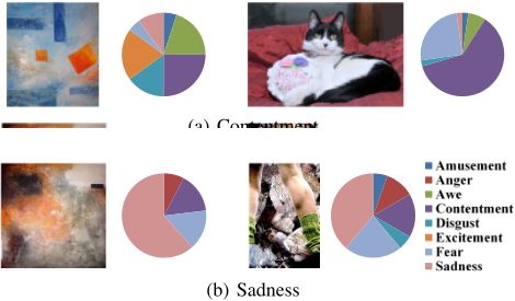
Specifically, effective hand-crafted or learning-based features have been designed to bridge the affective gap [Zhao et al., 2014a]. Existing IER methods mainly focused on assigning the dominant emotion category (DEC) or the average dimension values to an image, based on the assumption that viewers can reach a consensus on the emotion of images. However, labeling the emotions in images is in fact highly inconsistent, which causes the so-called subjective perception problem. That is, viewers might perceive different emotions from the same image due to the influence of various personal and situational factors, such as the cultural background, personality and social context [Joshi et al., 2011; Zhao et al., 2014a; Peng et al., 2015; Zhao et al., 2015b; Zhao et al., 2016]. Figure 1 illustrates the subjectivity issue for categorical emotions. To train an IER model, the emotion annotations need to be solicited from viewers. The groundtruth annotation of an image is usually obtained using the DEC. From Figure 1, we can see that the two images of each group differ a lot in terms of their emotion variances, even though they are with the same DEC.
As noted in [Zhao et al., 2016], to tackle the subjectivity challenge, two kinds of IER tasks can be performed: user-centric personalized emotion prediction for each viewer [Zhao et al., 2016] and image-centric emotion probability distribution prediction for each image [Zhao et al., 2015b; Peng et al., 2015; Zhao et al., 2017]. To address the issue of discrete probability distribution (DPD) modelling, shared sparse learning (SSL) [Zhao et al., 2015b], support vector regression (SVR) and convolutional neural network regression (CNNR) [Peng et al., 2015] were employed to learn the mapping between visual features and emotion probabilities. However, only uni-modal visual feature was considered in these methods, which is obviously insufficient, since image emotions are likely to be conveyed through complex visual features from low-level to high-level [Zhao et al., 2014b], such as color contrast and semantic concepts, as shown in Figure 1. In addition, the SVR and CNNR approaches do not guarantee that the predicted probability is non-negative.
In this paper, we propose a novel method to predict the DPD of image emotions from visual features, based on the following hypotheses:
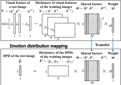
- Hypothesis 1: The images, which are jointly close to one another in the multi-modal visual feature space, would have similar DPDs in the categorical emotion space.
- Hypothesis 2: The DPD of a test image can be approximately modeled as a linear combination of the DPDs of the training images.
The proposed method, named weighted multi-modal shared sparse leaning (WMMSSL), mainly involves two processes, as illustrated in Figure 2. First, it learns a set of combination coefficients (called shared factors) to jointly reconstruct the multi-modal visual features of a test image with the features of the training images. Second, it linearly combines the DPDs using the shared factors leaned from the training images to compute the DPD of the test image. The two processes are referred to shared factors learning and emotion distribution mapping, respectively. The two special properties of WMMSSL lie in the exploration of representation abilities of different features and the automated weight learning for each feature in accordance with its importance. We validate the effectiveness of WMMSSL on Abstract [Machajdik and Hanbury, 2010], Emotion6 [Peng et al., 2015] and ImageEmotion-Social-Net [Zhao et al., 2016] datasets.
2 RelatedWork
Image emotion recognition. Categorical emotion states (CES) [Ekman, 1992; Mikels et al., 2005] and dimensional emotion space (DES) [Schlosberg, 1954] are two kinds of emotion representation models. Accordingly, different tasks can be performed, including affective image classification, regression and retrieval [Zhao et al., 2016].
Feature extraction plays an important role in IER. In the early years, different levels of hand-crafted features are designed to bridge the affective gap, including low-level color and texture [Machajdik and Hanbury, 2010], shape [Lu et al., 2012], mid-level principles-of-art [Zhao et al., 2014a] and high-level adjective noun pairs [Borth et al., 2013; Chen et al., 2014; Wang et al., 2016]. More recently, with the great success of convolutional nerual network (CNN) in many computer vision tasks, CNN has also been directly employed in IER [You et al., 2016b; Alameda-Pineda et al., 2016].
To learn the mapping between features and emotions, different machine learning methods have been employed, such as SVM [Lu et al., 2012], sparse learning [Zhao et al., 2017] and matrix completion [Alameda-Pineda et al., 2016].
Probability distribution prediction. In many machine learning applications, just predicting the most likely value for a target variable is not enough. For instance, in economics it is often important to study the fluctuation of stocks. In such cases, it would be more reasonable and useful to predict the probability distribution for that variable [Carney et al., 2005], such as surf height [Carney et al., 2005], user behavior [Liu et al., 2013] and spike events [Pipa et al., 2013]. As the emotions that are evoked in viewers by an image are highly subjective, predicting the distribution instead of the dominant emotion would make more sense. Generally, the distribution prediction task can be formalized as a regression problem. For CES, the task aims to predict the discrete probability of different emotion categories, the sum of which is equal to 1 [Zhao et al., 2015b; Peng et al., 2015]. For DES, the task usually turns to predicting the parameters of specified continuous probability distribution, such as Gaussian distribution [Zhao et al., 2015a; Zhao et al., 2017].
Sparse learning andmulti-modal learning. Sparse learning represents the target variable as a sparsely linear combination of a set of basis functions and is widely used in many areas, such as face recognition [Wright et al., 2009], visual classification [Yuan et al., 2012] and emotion analysis [Zhao et al., 2017]. Meanwhile, in many real-world applications, we might have multi-modal data [James and Dasarathy, 2014], either from different sources [You et al., 2016a] or with multiple features [Zhao et al., 2014b]. As different modal data usually represent different aspects of the target, jointly combining them may promisingly improve the performance [James and Dasarathy, 2014; Ding et al., 2016]. Besides the traditional early fusion and late fusion, there are many other multimodal fusion strategies, such as hypergraph learning [Zhou et al., 2006] and multimodal deep learning [Ngiam et al., 2011].
3 SystemOverview
Our goal is to predict the DPD of image emotions when multimodal features are available. Suppose we have L emotion categories c1, c2, · · · , cL and N training images I1, I2, · · · , IN. The mth modal features of the N training images are Xm = [xm1 , xm2 , · · · , xmN ] and the feature dimension is dm (m = 1, 2, · · · ,M). Let pn = [pn1, · · · , pnl, · · · , pnL]T denote the emotion distribution of the image In, where pnl represents the probability that image In conveys emotion cl (n = 1, 2, · · · ,N, l = 1, 2, · · · ,L). For each image In, we have ∑Ll=1 pnl = 1. Suppose I is a test image, its M modal features are y1 , y2 , · · · , yM and the ground-truth distribution is p = [p1, p2, · · · , pL]T. Let X = {X1 , X2 , · · · , XM } and Y = {y1 , y2 , · · · , yM } denote the feature set of the training images and the test image, respectively. Let P = [p1 , p2 , · · · , pN ] denote the training labels of emotion distribution. Then our task is to predict emotion distribution ̂p = [̂ p1, · · · , ̂ pl, · · · , ̂ pL]T, where ̂ pl = p(cl|Y) for test image I based on training examples (X, P). That is, our task aims to find the mapping
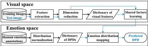
The framework of the proposed method is shown in Figure 3, which consists of operations in the visual space and the emotion space. In the visual space, we extract multi-modal features from the images and use PCA for dimension reduction. In the emotion space, the human emotion annotations are normalized to obtain the ground-truth DPDs for the training images. For a given test image, the shared factors learning algorithms are used to learn the mapping factors in the visual space, which are directly transferred to the emotion space to predict the DPD of the test image.
4 WeightedMulti-Modal Shared Sparse Learning
In practice, we can extract multi-modal visual features to represent images [Zhao et al., 2014b]. Jointly combining the strengths of multi-modal features may improve the performance of emotion distribution prediction. CNNR is based on CNN features, while SSL can simply adopt early or late fusion to handle multi-modal features without considering the latent correlations between different features. We present a weighted multi-modal shared sparse learning (WMMSSL) to provide additional useful information to the prediction problem by the constraint of joint sparsity across different features, which may enforce the robustness in coefficient estimation [Yuan et al., 2012].
WMMSSL assumes that multi-modal features Y and ̂p can be written in terms of bases X and P ∈ RL×N respectively, but with shared sparse coefficients Θ ∈ RN×M . That is
where Θ = [θ1 , θ2 , · · · , θM ] and w = [w1, w2, · · · , wM]T are obtained by
where α and β are regularization coefficients that control the relative importance of the regularization terms and the sumof-squares error term. The constraints θm ≥ 0, ‖θm‖1 = 1 and w ≥ 0, ‖w‖1 = 1 together ensure that the predicted ̂p is a probability distribution.
To solve the dual-optimization problem in Eq. (3), we alternatively conduct optimization.
(1) Updating Θ when fixing w
We employ IRLS [Chartrand and Yin, 2008] to optimize Θ in Eq. (3), the component ‖Θ‖2,1 of which is transformed by
where ε > 0 is introduced to avoid division by zero. Let ϕn = 1/(√∑M m=1 (θm n )2 + ε). Define diagonal matrix Φ(n, n) = √ϕn(1 ≤ n ≤ N). Then the objective function of Eq. (3) with respect to Θ is transformed to
minO(Θ) can be optimized for each θm independently
which can be easily and efficiently solved by off-the-shelf quadratic optimization methods.
(2) Updating w when fixing Θ
The optimization problem of Eq. (3) with respect to w is transformed to
which is a also quadratic programming problem. The learning procedure is summarized in Algorithm 1. The computation complexity is O(c · M · E · N 2 ), where c is the number of iterations in conjugate gradient when optimizing θm.
Algorithm 1: Procedure for weighted multi-modal shared sparse leaning
Input: Training examples (X, P), test feature Y, max-epochs E, error threshold τ1, τ2, regularization coefficients α, β Output: Predicted emotion distribution ̂p for Y 1 Initialization: θm(0) ← 1/N(m= 1, 2, · · · ,M), ε ← 10-9 , p ← 0, w(0) ← 1/M; 2 for e ← 1 to E do /* Updating Θ when fixing w */ 3 for m ← 1 to M do 4 Compute the diagonal matrix Φ(e) by ϕ(e) n ← 1/(√∑M m=1 (θm(e-1) n )2 + ε), Φ(e) (n, n) ← √ϕ(e) n (1 ≤ n ≤ N); 5 Optimize θm by θm(e) ← argmin w(e-1) m ‖ym -Xmθm‖22 +α‖Φ(e)θm‖22, s.t. θm ≥ 0, ‖θm‖1 = 1; 6 7 end /* Updating w when fixing Θ */ 8 Optimize w by w(e) ← argmin ∑M m=1 wm‖ym - Xmθm(e) ‖22 + β‖w‖22, s.t. w ≥ 0, ‖w‖1 = 1; 9 10 if ‖θm(e) - θm(e-1) ‖2 < τ1(m = 1, 2, · · · ,M) & ‖w(e) -w(e-1) ‖2 < τ2 then 11 break; 12 end 13 end 14 Θ(e) = [θ1(e) , θ2(e) , · · · , θM(e) ]; 15 return ̂p = PΘ(e)w(e) .5 Experiments
To our knowledge, there are three public datasets that contain DPD information of image emotions: Abstract [Machajdik and Hanbury, 2010], Emotion6 [Peng et al., 2015] and ImageEmotion-Social-Net (IESN) [Zhao et al., 2016]. In this section, we introduce the experimental settings and evaluate the performance of the proposed method.
5.1 Experimental Settings
Datasets: The Abstract dataset [Machajdik and Hanbury, 2010] includes 279 abstract paintings without any recognizable objects. These images were peer rated in a websurvey by approximately 230 people into 8 emotion categories [Mikels et al., 2005]. On average each image was rated about 14 times. Only 228 images can be used for affective image classification [Machajdik and Hanbury, 2010], while all the images can be used for emotion distribution prediction.
The Emotion6 dataset [Peng et al., 2015] consists of 1,980 images collected from Flickr, 330 for each of the Ekman's 6 basic emotions [Ekman, 1992]. The emotional responses from subjects were obtained using Amazon Mechanical Turk
(AMT). Each image was scored by 15 subjects into Ekman's 6 basic emotions and neutral.
The IESN dataset [Zhao et al., 2016] contains 1,012,901 images collected from Flickr using keywords based searching strategy [Borth et al., 2013]. The emotion information of the social images in IESN are automatically obtained from the text data. Similar to Abstract [Machajdik and Hanbury, 2010], the emotions are also classified into 8 categories. Totally, we select 3,792 images, each of which is assigned with more than 15 categorial emotion labels.
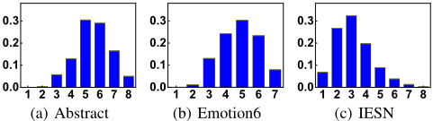
The emotion distribution on the 8 or 7 categories of each image can be easily obtained by normalization, i.e., dividing the number of subjects who perceive each emotion category by the number of all emotion perceptions. For example, given an image, suppose the perceived emotion number by 20 subjects on the 8 emotion categories is v = [7, 0, 4, 5, 0, 6, 2, 1], then the DPD is v/ ∑(v) = [0.28, 0, 0.16, 0.2, 0, 0.24, 0.08, 0.04]. Note that one subject can perceive multiple emotions from the same image. The distribution of emotion numbers for the images in the three datasets is shown in Figure 4, from which we can clearly see the subjectivity issue of emotion perceptions.
Emotion Features: To enhance the representation power, we extract various features, including hand-crafted ones of different levels and learning-based ones.
We first extract two classes of low-level hand-crafted features for their global descriptors of the overall image content, including GIST [Patterson and Hays, 2012] and the features derived from elements-of-art (color and texture) [Machajdik and Hanbury, 2010]. Mid-level features are more interpretable and have stronger link to emotions than low-level ones [Zhao et al., 2014a]. Here we extract two classes of mid-level features, including attributes [Patterson and Hays, 2012] and features inspired from principles-of-art [Zhao et al., 2014a]. High-level features reflect the semantic contents in images. We extract a set of concepts described by adjective noun pairs (ANPs), which are detected by a large detector library SentiBank [Borth et al., 2013]. Further, we extract the deep learning features from the response of the fully connected layer (FC) 7 of the ImageNet-CNN [Krizhevsky et al., 2012], which is the final fully connected layer before producing the class predictions. The six sets of extracted features are abbreviated as GIST, Elem, Attr, Prin, ANP and CNN with dimension 512, 48, 102, 165, 1200 and 4096, respectively.
| SSL-GIST | SSL-Elem | SSL-Attr | SSL-Prin | SSL-ANP | SSL-CNN | CNNR | SSL-Early | SSL-Late | WMMSSL | |
|---|---|---|---|---|---|---|---|---|---|---|
| SSD | 1.369±0.073 | 1.354±0.134 | 1.473±0.090 | 1.346±0.106 | 1.316±0.035 | 1.282±0.046 | 1.244±0.096 | 1.271±0.045 | 1.241±0.055 | 1.191±0.060 |
| KL | 5.525±0.329 | 5.439±1.379 | 6.070±0.204 | 5.421±0.551 | 5.475±0.153 | 5.225±0.177 | 5.103±0.305 | 5.126±0.096 | 5.034±0.177 | 4.820±0.209 |
| BC | 7.992±0.108 | 8.095±0.168 | 7.849±0.928 | 8.106±0.077 | 8.118±0.048 | 8.118±0.074 | 8.173±0.093 | 8.142±0.046 | 8.210±0.081 | 8.319±0.078 |
| R2 | 1.915±0.236 | 2.161±0.372 | 1.850±0.395 | 2.478±0.428 | 2.483±0.337 | 2.660±0.385 | 2.796±0.309 | 2.678±0.354 | 2.818±0.456 | 2.993±0.467 |
| SSL-GIST | SSL-Elem | SSL-Attr | SSL-Prin | SSL-ANP | SSL-CNN | CNNR | SSL-Early | SSL-Late | WMMSSL | |
|---|---|---|---|---|---|---|---|---|---|---|
| SSD | 2.043±0.061 | 1.828±0.061 | 1.984±0.033 | 1.806±0.065 | 1.794±0.122 | 1.427±0.043 | 1.394±0.080 | 1.344±0.033 | 1.402±0.086 | 1.268±0.076 |
| KL | 6.389±0.317 | 5.999±0.882 | 6.205±0.096 | 5.863±0.445 | 5.705±0.306 | 5.244±0.041 | 4.846±0.469 | 4.825±0.084 | 5.064±0.150 | 4.793±0.097 |
| BC | 7.868±0.097 | 7.940±0.049 | 7.909±0.009 | 8.111±0.113 | 8.151±0.061 | 8.402±0.015 | 8.437±0.050 | 8.484±0.012 | 8.411±0.044 | 8.529±0.059 |
| R2 | 2.755±0.381 | 3.601±0.104 | 2.832±0.151 | 3.644±0.117 | 3.683±0.182 | 4.237±0.014 | 4.434±0.348 | 4.533±0.180 | 4.368±0.161 | 4.679±0.172 |
| SSL-GIST | SSL-Elem | SSL-Attr | SSL-Prin | SSL-ANP | SSL-CNN | CNNR | SSL-Early | SSL-Late | WMMSSL | |
|---|---|---|---|---|---|---|---|---|---|---|
| SSD | 1.928±0.431 | 1.854±0.078 | 1.863±0.008 | 1.852±0.113 | 1.728±0.002 | 1.719±0.054 | 1.703±0.022 | 1.676±0.125 | 1.706±0.090 | 1.569±0.014 |
| KL | 5.606±1.136 | 5.292±0.385 | 5.173±0.177 | 5.083±0.929 | 4.915±0.288 | 4.874±0.115 | 4.828±0.953 | 4.812±0.108 | 4.837±0.134 | 4.777±0.016 |
| BC | 8.450±0.290 | 8.456±0.054 | 8.461±0.020 | 8.486±0.055 | 8.505±0.003 | 8.515±0.037 | 8.534±0.047 | 8.542±0.072 | 8.525±0.068 | 8.583±0.015 |
| R2 | 6.828±0.361 | 7.043±0.059 | 7.154±0.283 | 7.201±0.501 | 7.221±0.319 | 7.232±0.239 | 7.306±0.015 | 7.314±0.178 | 7.265±0.171 | 7.358±0.382 |
Baselines: Shared sparse learning (SSL) [Zhao et al., 2015b] and convolutional neural network regression (CNNR) [Peng et al., 2015] are selected as baselines for comparison. Besides each uni-modal feature, we also implement early and late fusion for SSL to handle multi-modal features. The settings of CNNR is similar to [Peng et al., 2015], where the Caffe reference model [Jia et al., 2014] is pre-trained and the CNN is fine-tuned with our training set.
Evaluation Metrics: The sum of squared difference (SSD) [Zhao et al., 2015b], the Kullback-Leibler divergence (KL), the Bhattacharyya coefficient (BC) and the coefficient of determination (R2 ) are used as evaluation metrics. 0 ≤ SSD ≤ 1, KL ≥ 0 and lower values indicate better performance. 0 ≤ BC ≤ 1 and larger value represents better results. R2 ranges from 0 to 1 and larger value represents stronger linear relationship between two distributions. Please note that (1) SSD measures the performance from the aspect of regression, while KL, BC and R2 measure the distance between two distributions; (2) KL and BC emphasize on each individual element, whereas R2 considers the variance among all the elements in the DPD.
Implementation Details: We randomly select 80%, 50% and 50% of images from the Abstract, Emotion6 and IESN datasets respectively as the training set and the remained form the testing set. The following parameter settings are adopted for WMMSSL: α = 0.05 and β = 0.1. We also conduct empirical analysis on parameter sensitivity, which demonstrates that WMMSSL has superior and stable performance with a wide range of parameter values on all three datasets. The features that are over 50-dimensional are all reduced to 50 by PCA to accelerate the optimization. For better comparison, the parameters of the baselines are carefully tuned and the best results are reported. To remove the influence of any randomness, we perform 20 runs and report the average results and the standard deviation.
5.2 Results and Discussion
On Uni-Modal Visual Features
Firstly, we conduct experiments to compare the performance of different visual features and uni-modal feature based methods, i.e. SSL [Zhao et al., 2015b] and CNNR [Peng et al., 2015], for emotion distribution prediction. The performances measured by SSD, KL, BC, R2 and the standard deviations on Abstract, Emotion6 and IESN datasets are summarized in Table 1, Table 2 and Table 3, respectively. In the middle column of each table, the best uni-modal feature based method is highlighted in italic.
From the results, we have the following observations. (1) Generally, the CNN features have stronger discriminability than the hand-crafted ones; the high-level and mid-level hand-crafted features perform better than low-level ones. Theses results are consistent with several existing literatures [You et al., 2016b; Zhao et al., 2016; Zhao et al., 2014b]. (2) The CNNR method achieves the best results in most cases with uni-modal features, which demonstrates the effectiveness of CNNR in DPD prediction of image emotions [Peng et al., 2015]. (3) The metrics SSD, KL, BC and R2 relatively comply with the performance measure of emotion distribution prediction.
Besides the common observations above, there are some inconsistencies across datasets. (1) The features derived from principles-of-art and elements-of-art perform even better than the high-level ANP features on Abstract and Emotion6 datasets. This is probably because the images in Abstarct are abstract paintings without recognizable objects, the emotions of which are mainly evoked by art theory and aesthetics. Meanwhile, the apparent semantics directly related to the evoked emotions, such as expressive faces, are removed in the Emotion6 dataset construction [Peng et al., 2015]. (2) The metric R2 is much larger in IESN dataset than Abstract and Emotion6 datasets, since the evoked emotion numbers of each image is smaller in IESN (Figure 4) due to the influence of social factors, such as the joined interest groups.


On Different Feature Fusion Methods
Secondly, we compare the performance of different feature fusion methods for emotion distribution prediction, including the proposed WMMSSL, early fusion and late fusion for SSL. The results are reported in the right column of Table 1, Table 2 and Table 3, where the better fusion method for SSL is shown in bold, while the best overall result is highlighted in both italic and bold.
Comparing the results, we can observe that: (1) fusing multi-modal features by either early fusion or late fusion for SSL can obtain better prediction performance than most unimodal features; (2) the best fusion method for SSL is dependent on the datasets; on Abstract dataset, late fusion achieves better performance, while early fusion works better on Emotion6 and IESN datasets; (3) SSL with late, early and early fusion method outperforms CNNR on Abstract, Emotion6 and IESN datasets, respectively; (4) the proposed fusion method, namely WMMSSL, performs the best on the three datasets, which demonstrates the effectiveness of WMMSSL for emotion distribution prediction.
Specifically, the performance gains of SSL with the best fusion method over the best uni-modal features measured by SSD, KL, BC, R2 are 3.20%, 3.66%, 1.13%, 5.94% on Abstract, 5.82%, 7.99%, 0.98%, 6.99% on Emotion6 and 2.50%, 1.48%, 0.32%, 1.13% on IESN datasets, respectively. Compared with the best results of CNNR and SSL, the proposed WMMSSL achieves the KL performance gains of 5.55%, 4.25% on Abstract, 1.09%, 0.66% on Emotion6 and 1.06%, 0.73% on IESN datasets, respectively. These results demonstrate that the proposed WMMSSL outperforms the state-ofthe-art approaches for emotion distribution prediction with significant performance gains.
On Parameter Sensitivity
In WMMSSL, we have two model parameters, α to control the model sparsity and β as the feature weight parameter. We investigate how sensitive WMMSSL is to the parameters. When analyzing α and β, we fix the other as the value we introduced above.
The influences of the regularization parameters α, β on WMMSSL are validated, with results shown in Figure 5 and Figure 6. From these results, we can find that: (1) the influences of α, β are different on different datasets; more stable performances are obtained on Emotion6 and IESN datasets than Abstract dataset; (2) generally, with the decrease of α, the performance tends to become better with relatively stable performance achieved when α decreases to 0.1; (3) on Abstract dataset, with the increase of β, the performance firstly becomes better and then turns to be worse, meaning that there exists the best β; though not so obviously, WMMSSL achieves better KL values when β ≥ 0.1 on Emotion6 and IESN datasets. These results reveal the robustness of the proposed method for emotion distribution prediction.
6 Conclusion
In this paper, we proposed a novel method, named weighted multi-modal shared sparse leaning, to predict the discrete probability distribution of image emotions. Features from different modalities, both hand-crafted ones and learning-based ones, are jointly explored. The optimal weights for different features that reflect their representation abilities are automatically learned from the training data. Experiments on Abstract, Emotion6 and IESN datasets demonstrated the effectiveness of WMMSSL. For future studies, we plan to improve the computational efficiency of WMMSSL to tackle largescale data. Further, we will implement applications based on emotion distribution, such as affective image retrieval.
@inproceedings{ijcai2017p651,
  title     = {Approximating Discrete Probability Distribution of Image Emotions by Multi-Modal Features Fusion},
  author    = {Zhao, Sicheng and Ding, Guiguang and Gao, Yue and Han, Jungong},
  booktitle = {Proceedings of the Twenty-Sixth International Joint Conference on
               Artificial Intelligence, {IJCAI-17}},
  publisher = {International Joint Conferences on Artificial Intelligence Organization},
  editor    = {Carles Sierra, IIIA-CSIC},
  pages     = {4669--4675},
  year      = {2017},
  month     = {8},
  note      = {Main track},
  doi       = {10.24963/ijcai.2017/651},
  url       = {https://doi.org/10.24963/ijcai.2017/651},
}
TY - CPAPER TI - Approximating Discrete Probability Distribution of Image Emotions by Multi-Modal Features Fusion AU - Zhao, Sicheng AU - Ding, Guiguang AU - Gao, Yue AU - Han, Jungong T2 - Proceedings of the Twenty-Sixth International Joint Conference on Artificial Intelligence, IJCAI-17 PB - International Joint Conferences on Artificial Intelligence Organization PY - 2017 SP - 4669 EP - 4675 DO - 10.24963/ijcai.2017/651 UR - https://doi.org/10.24963/ijcai.2017/651 ER -Copied
Machine-readable versions of this paper, for tools and AI agents:





