
An ASP Approach to Generate Minimal Countermodels in Intuitionistic Propositional Logic
Proceedings of the Twenty-Eighth International Joint Conference on Artificial Intelligence. Main track. Pages 1675-1681.
https://doi.org/10.24963/ijcai.2019/232
Keywords
- Heuristic Search and Game Playing: Modeling
- Knowledge Representation and Reasoning: Automated Reasoning and Theorem Proving
Abstract
Intuitionistic Propositional Logic is complete w.r.t. Kripke semantics: if a formula is not intuitionistically valid, then there exists a finite Kripke model falsifying it. The problem of obtaining concise models has been scarcely investigated in the literature. We present a procedure to generate minimal models in the number of worlds relying on Answer Set Programming (ASP).
- [Baral, 2010] Chitta Baral. Knowledge Representation, Rea- soning and Declarative Problem Solving. Cambridge Uni- versity Press, 2010.
- [Bry and Yahya, 2000] Franc ¸ois Bry and Adnan H. Yahya. Positive unit hyperresolution tableaux and their applica- tion to minimal model generation. J. Autom. Reasoning, 25(1):35-82, 2000.
- [Chagrov and Zakharyaschev, 1997] Alexander V. Chagrov and Michael Zakharyaschev, Modal Logic. Oxford Uni- versity Press, 1997.
- [Cheney et al., 2016] James Cheney, Alberto Momigliano, and Matteo Pessina. Advances in Property-Based Testing for αProlog. In TAP, volume 9762 of LNCS, pages 37-56. Springer, 2016.
- [Claessen and Rosén, 2015] Koen Claessen and Dan Rosén. SAT modulo intuitionistic implications. In M. Davis et al., editors., LPAR-20, Proceedings, volume 9450 of LNCS, pages 622-637. Springer, 2015.
- [Corsi and Tassi, 2007] Giovanna Corsi and Gabriele Tassi. Intuitionistic logic freed of all metarules. J. Symb. Log., 72(4):1204-1218, 2007.
- [Dantsin et al., 2001] Evgeny Dantsin, Thomas Eiter, Georg Gottlob, and Andrei Voronkov. Complexity and expres- sive power of logic programming. ACM Comput. Surv., 33(3):374-425, 2001.
- [Demri et al., 2014] Stéphane Demri, Deepak Kapur, and Christoph Weidenbach, editors. IJCAR 2014, Proceedings, volume 8562 of LNCS. Springer, 2014.
- [Dummett, 1959] Michael Dummett. A propositional calcu- lus with denumerable matrix. J. Symbolic Logic, 24(2):97- 106, 1959.
- [Dyckhoff, 2016] Roy Dyckhoff. Intuitionistic decision pro- cedures since Gentzen. In Advances in proof theory, vol- ume 28 of Progr. Comput. Sci. Appl. Logic, pages 245- 267. Birkhäuser/Springer, [Cham], 2016.
- [Ferrari et al., 2013] Mauro Ferrari, Camillo Fiorentini, and Guido Fiorino. Contraction-free linear depth sequent cal- culi for intuitionistic propositional logic with the subfor- mula property and minimal depth counter-models. J. Au- tom. Reasoning, 51(2):129-149, 2013.
- [Ferrari et al., 2015] Mauro Ferrari, Camillo Fiorentini, and Guido Fiorino. An evaluation-driven decision procedure for G3i. ACM Trans. Comput. Log., 16(1):8:1-8:37, 2015.
- [Fiorentini and Ferrari, 2017] Camillo Fiorentini and Mauro Ferrari. A forward unprovability calculus for intuitionis- tic propositional logic. In R. A. Schmidt and C. Nalon, editors, TABLEAUX 2017, volume 10501 of LNCS, pages 114-130. Springer, 2017.
- [Galmiche and Larchey-Wendling, 1999] Didier Galmiche and Dominique Larchey-Wendling. Structural sharing and efficient proof-search in propositional intuitionistic logic.
- In P. S. Thiagarajan et al., editors, Advances in Computing Science -ASIAN'99, Proceedings, volume 1742 of LNCS, pages 101-112. Springer, 1999.
- [Gebser et al., 2011] Martin Gebser, Benjamin Kaufmann, Roland Kaminski, Max Ostrowski, Torsten Schaub, and Marius Thomas Schneider. Potassco: The Potsdam An- swer Set Solving Collection. AI Commun., 24(2):107-124, 2011.
- [Gebser et al., 2012] Martin Gebser, Roland Kaminsk, Ben- jamin Kaufmann, and Torsten Schaub. Answer Set Solving in Practice. Synthesis Lectures on Artificial Intelligence and Machine Learning. Morgan and Claypool Publishers, 2012.
- [Goré and Thomson, 2012] Rajeev Goré and Jimmy Thom- son. Bdd-based automated reasoning for propositional bi- intuitionistic tense logics. In B. Gramlich et al., editors, IJCAR 2012, Proceedings, volume 7364 of LNCS, pages 301-315. Springer, 2012.
- [Goré et al., 2014] Rajeev Goré, Kerry Olesen, and Jimmy Thomson. Implementing tableau calculi using bdds: Bd- dtab system description. In Demri et al. [2014], pages 337-343.
- [Larchey-Wendling et al., 2001] Dominique Larchey- Wendling, Dominique Méry, and Didier Galmiche. STRIP: Structural Sharing for Efficient Proof-Search. In R. Goré et al., editors, IJCAR 2001, Proceedings, volume 2083 of LNCS, pages 696-700. Springer, 2001.
- [Lorenz, 1994] Sven Lorenz. A tableaux prover for domain minimization. J. Autom. Reasoning, 13(3):375-390, 1994.
- [Negri, 2014] Sara Negri. Proofs and countermodels in non- classical logics. Logica Universalis, 8(1):25-60, 2014.
- [Niemelä, 1996] Ilkka Niemelä. A tableau calculus for min- imal model reasoning. In P. Miglioli et al., editors, TABLEAUX '96, Proceedings, volume 1071 of LNCS, pages 278-294. Springer, 1996.
- [Papacchini and Schmidt, 2011] Fabio Papacchini and Re- nate A. Schmidt. A tableau calculus for minimal modal model generation. Electr. Notes Theor. Comput. Sci., 278:159-172, 2011.
- [Papacchini and Schmidt, 2014] Fabio Papacchini and Re- nate A. Schmidt. Terminating minimal model generation procedures for propositional modal logics. In Demri et al. [2014], pages 381-395.
- [Pearce, 1997] David Pearce. A new logical characterisation of stable models and answer sets. In J. Dix et al., editors, Non-Monotonic Extensions of Logic Programming, pages 57-70, Berlin, Heidelberg, 1997. Springer Berlin Heidel- berg. [Pinto and Dyckhoff, 1995] Luis Pinto and Roy Dyckhoff. Loop-free construction of counter-models for intuitionis- tic propositional logic. In Behara et al., editor, Sym- posia Gaussiana, Conference A, pages 225-232.
- [Raths et al., 2007] Thomas Raths, Jens Otten and Christoph Kreitz. The ILTP problem library for intuitionistic logic. J. Autom. Reasoning, 31:261-271, 2007.
- [Skura, 2011] Tomasz Skura. Refutation Systems in Propo- sitional Logic. In D. Gabbay et al., editors, Handbook of Philosophical Logic, volume 16, pages 115-157. Springer, Dordrecht, 2011.
- [Svejdar, 2006] Vítezslav Svejdar. On sequent calculi for intuitionistic propositional logic. Comment. Math. Univ. Carolinae, 47(1):159-173, 2006.
References were extracted automatically from the PDF and may contain errors.
Full text extracted automatically from the PDF; figures, tables and equations may differ. The PDF is the version of record.
1 Introduction
Intuitionistic Propositional Logic (IPL) has the finite model property w.r.t. Kripke semantics: if a formula G is not valid in IPL, then G can be falsified in a finite (Kripke) model K; we call K a countermodel for G. In many of the proofsearch strategies for IPL (see [Dyckhoff, 2016] for a review), whenever the search for a derivation of a formula G fails, a countermodel for G is provided. A countermodel can be understood as a "certificate" witnessing the non-validity of the formula G, thus countermodels can be used for diagnosis, to analyze why some property fails or to fix errors in formal specifications. This methodology has been successfully applied to Property-Based Testing (PBT), where the user defines a property that the code to be checked is expected to fulfill and the PBT engine generates test cases to validate it; failing cases (countermodels) detect flaws and are exploited to amend the code (see, e.g., [Cheney et al., 2016] for an application to αProlog). In this perspective, it is critical that countermodels are minimal so as to convey a plain and concise representation of non-validity. For classical logics, various notions of minimality have been introduced, aiming at reducing the domain of interpretations (e.g. [Lorenz, 1994]) or the interpretation of predicates (e.g. [Niemel¨a, 1996; Bry and Yahya, 2000]). For modal and description logics, a semantic notion of minimality based on subset-simulation has been proposed in [Papacchini and Schmidt, 2011; 2014], where terminating procedures to build minimal models for some of the logics between K and S5 are presented.
Here we aim at minimizing the size of countermodels, measured by the number of worlds: a countermodel K for G is minimal if no countermodel for G has size less then the size of K (thus, if G is not classically valid, the minimal countermodel only contains a world). This issue has been scarcely investigated in the literature, where the emphasis is mainly on derivations, and countermodels are often obtained as a byproduct (see, e.g., [Pinto and Dyckhoff, 1995; Corsi and Tassi, 2007; Negri, 2014; Claessen and Ros´en, 2015]). Also the known refutation calculi for IPL, namely the calculi designed to prove the non-validity of formulas (see, e.g., [Skura, 2011]), do not focus on the size of countermodels. More relevant to this issue are the proof-search procedures described in [Galmiche and Larchey-Wendling, 1999; Larchey-Wendling et al., 2001; Svejdar, 2006; Ferrari et al., 2013; 2015; Fiorentini and Ferrari, 2017], which yield models having depth bounded by the goal formula; however, minimality of countermodels is not ensured. One might naively guess that it is always possible to shrink a given countermodel, for instance by using the filtration techniques discussed in [Chagrov and Zakharyaschev, 1997]; actually, it is unlikely that such a general method exists (see Sec. 3).
To tackle the problem, we propose a quite different strategy, based on model generation: given a goal formula G, we try to build a countermodel for G by a model-search procedure guided by semantics. A naive implementation of the process immediately blows-up and, even for small goal formulas, model generation is not terminating; thus, we need a clever formalization of the problem. Following [Gor´e and Thomson, 2012; Gor´e et al., 2014], worlds of models are represented by sets W of atomic subformulas H of G (namely: H is either a propositional variable or H = ¬A or H = A → B) satisfying some closure properties. The first selected set W is a putative world falsifying G. To get a well-defined Kripke model, we have to guarantee that atomic subformulas of G not belonging to W are not valid in W. For instance, if A → B ̸∈ W, we need a world Z such that Z is a successor of W (namely, W ⊆ Z) and Z witnesses the non-validity of A → B in W (namely, A holds in Z and B does not hold). This triggers a saturation process which successfully ends when all the needed witnesses have been generated, thus yielding a countermodel for G.
We formalize the problem in Answer Set Programming (ASP) [Baral, 2010], a form of declarative programming based on the stable model semantics (answer sets), which enables to solve hard search problems in a uniform way [Dantsin et al., 2001]. We define an ASP program ΠG such that an answer set of ΠG corresponds to a countermodel for G; if no answer exists, there is no countermodel for G, meaning that G is valid (in IPL). To compute answer sets, we exploit the Potassco tool clingo [Gebser et al., 2011]. The minimization of models is delegated to clingo; however, it is critical to encode the problem so that even the first computed model is small, otherwise the minimization engine gets stuck. Differently from other declarative formalisms, ASP allows for a quite modular formalization; as outlined in Sec. 4, the generator can be easily extended to deal with intermediate logics where the frame conditions can be expressed in ASP, such as G¨odel-Dummett logic [Dummett, 1959] and Here and There logic [Pearce, 1997]. The implementation is available at author's home page.
2 Minimal Countermodels in IPL
We consider the propositional language L based on a denumerable set of propositional variables V and the connectives ¬, ∧, ∨, →. Let A be a formula. By Sf(A) we denote the set of all subformulas of A. The size of A, denoted by |A|, is the number of symbols occurring in A. A (Kripke) model is a triple 〈P,≤, V 〉, where 〈P,≤〉 is a finite poset and V (the evaluation function) is a monotone map P → 2V , namely: w ≤ w′ implies V (w) ⊆ V (w′ ); elements of P are called worlds. The forcing relation ⊩⊆ P × L is defined as usual:
Note that ⊩ is monotone, namely: w ⊩ A and w ≤ w′ implies w′ ⊩ A. If Γ is a set of formulas, by w ⊩ Γ we mean w ⊩ A for every A ∈ Γ. A formula G is valid in IPL iff, for every model K and world w of K, w ⊩ G. Thus, to certify that G is not valid (in IPL) we can exhibit a model K containing a world w such that w ⊮ G; we call K a countermodel for G. We aim at representing worlds of K by means of proper subsets W of Sf(G). To avoid redundancies, we consider sets W only containing subformulas H of G of the form H ∈ V or H = ¬A or H = A → B; we call H an atomic subformula of G and by At(G) we denote the set of all atomic subformulas of G. By ClG(W) we denote the smallest set satisfying the following properties, where -(¬A) = A and -A = ¬A if A ̸= ¬B:
- W ⊆ ClG(W) ⊆ Sf(G).
- C = A ∧ B ∈ Sf(G) and {A,B} ⊆ ClG(W) implies C ∈ ClG(W).
- C = A∨B ∈ Sf(G) and {A, B}∩ClG(W) ̸= ∅ implies C ∈ ClG(W).
- C = A → B ∈ Sf(G) and {-A,B} ∩ ClG(W) ̸= ∅ implies C ∈ ClG(W).
- C = ¬¬A ∈ Sf(G) and A ∈ ClG(W) implies C ∈ ClG(W).
- C = ¬(A∧B) ∈ Sf(G) and {-A, -B}∩ClG(W) ̸= ∅ implies C ∈ ClG(W).
- C = ¬(A ∨ B) ∈ Sf(G) and {-A,-B} ⊆ ClG(W) implies C ∈ ClG(W).
Figure 1: The formula T and the related p-worlds W0, . . . ,W9
- C = ¬(A → B) ∈ Sf(G) and {A,-B} ⊆ ClG(W) implies C ∈ ClG(W).
By induction on formulas, we can prove that:
A set W ⊆ At(G) is a p-world (possible world) iff it satisfies the following closure properties:
In the ASP representation, we limit ourselves to use p-worlds as candidate worlds of countermodels; as shown in the examples, this considerably reduces the number of subsets of At(G) to be considered in model generation.
Example 1 Let T be the non-valid formula defined in Fig. 1 (T is equivalent to Nishimura formula N9, see Ex. 7). Then:
- Z0 = At(T) satisfies the closure properties (C →) and (CAt), but not (C¬), since ¬¬p ∈ Z0 and ¬p ∈ ClT (Z0).
- Z1 = {S, T} satisfies (C¬) and (CAt), but not (C→), since T ∈ Z1, S ∈ ClT (Z1) and X ∨ ¬¬p ̸∈ ClT (Z1).
- Let Z2 = {¬p, X → D, S, T}. Since -(¬¬p) = ¬p ∈ Z2, then X ∈ ClT (Z2). This implies that Z2 satisfies (C¬) and (C→) but not (CAt).
The set At(T) contains 7 elements, giving rise to 27 = 128 subsets, but only 10 of them are p-worlds, namely the sets W0, . . . ,W9 displayed in Fig. 1. ✸
This representation is close to [Gor´e and Thomson, 2012], with some tweak. We treat ¬ as a primitive connective (thus, ¬p is not an abbreviation for p → ⊥) and, in the definition of ClG(W), negated formulas are analyzed according to the constructive interpretation of ¬. This reduces the number of p-worlds; for instance, in Ex. 1 we keep out p-worlds W such that p ∈ W and ¬¬p ̸∈ W.
Let P be a set of p-worlds; by K(P) we denote the model 〈P,≤, V 〉 such that ≤ coincides with the subset relation ⊆ and, for every W ∈ P , V (W) = W ∩ V. In general W does not coincide with the set of atomic subformulas of G forced at W. For instance, it might happen that A → B ̸∈ W, but there is no Z ∈ P witnessing that W ⊮ A → B, namely: W ≤ Z and Z ⊩ A and Z ⊮ B. To get a close correspondence between membership and forcing we introduce the notion of G-saturation. A set of p-worlds P is G-saturated iff, for every W ∈ P , the following saturation properties hold:
- (S1) for every ¬A ∈ At(G) \ W, there is Z ∈ P such that W ⊆ Z and A ∈ ClG(Z).
- (S2) For every A → B ∈ At(G) \W, there is Z ∈ P such that W ⊆ Z and A ∈ ClG(Z) and B ̸∈ ClG(Z).
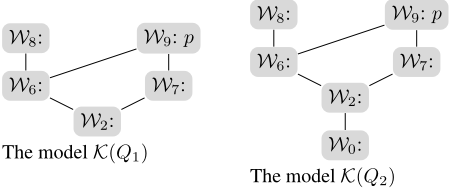
Example 2 (Ex. 1 cont) The sets below are T-saturated:
For instance, we have X = ¬¬p → p ̸∈ W2 and (S2) is matched by setting Z = W7. The models K(Q1) and K(Q2) are displayed in Fig. 2; for each world Wk, we list the propositional variables in Wk. In both models, for every H ∈ At(T), Wk ⊩ H iff H ∈ Wk (see next lemma), accordingly W2 ⊮ T . ✸
Lemma 1 Let P be a G-saturated set. For every W ∈ P and A ∈ Sf(G), W ⊩ A in K(P ) iff A ∈ ClG(W).
Proof: Let K(P) = 〈P, ≤, V 〉, W ∈ P and A ∈ Sf(G); we prove the lemma by induction on |A|; we only detail some representative case. Let A = ¬B (thus ¬B ∈ At(G)). If ¬B ̸∈ ClG(W), then ¬B ̸∈ W hence, by (S1), there is Z ∈ P such that W ⊆ Z and B ∈ ClG(Z). By (IH), Z ⊩ B; since W ≤ Z, we conclude W ⊮ ¬B. Conversely, let W ⊮ ¬B. Then, there is Z ∈ P such that W ≤ Z and Z ⊩ B; by (IH), B ∈ ClG(Z). Since Z satisfies (C¬), ¬B ̸∈ Z. Since W ⊆ Z, we get ¬B ̸∈ W and, by (CAt), we conclude ¬B ̸∈ ClG(W). Let A = B0 ∨ B1. If W ⊩ B0 ∨ B1, then W ⊩ Bk, with k ∈ {0, 1}. By (IH), Bk ∈ ClG(W), which implies B0 ∨ B1 ∈ ClG(W). Conversely, if B0 ∨ B1 ∈ ClG(W), then Bk ∈ ClG(W), with k ∈ {0, 1}. By (IH), W ⊩ Bk, hence W ⊩ B0 ∨ B1. ♦
Lemma 2 Let K = 〈P, ≤, V 〉 be a model and G a formula. Then, there exist a G-saturated set Q and a surjective map φ : P → Q such that, for every w ∈ P and A ∈ Sf(G), w ⊩ A iff A ∈ ClG(φ(w)).
Proof: Let φ be the map from P to 2At(G) defined as
and w ∈ P ; we prove that:
- for every A ∈ Sf(G), w ⊩ A iff A ∈ ClG(φ(w)).
- φ(w) is a p-world.
Since w ⊩ φ(w), by (P2) we get w ⊩ ClG(φ(w)), and this proves the if part of (1). Conversely, let A ∈ Sf(G) such that w ⊩ A; by induction on |A| one can easily show that A ∈ ClG(φ(w)), and this proves (1). Let ¬A ∈ φ(w); then w ⊩ ¬A, hence w ⊮ A. By (1), A ̸∈ ClG(φ(w)), hence φ(w) satisfies (C¬). The proof that φ(w) matches both (C→) and (CAt) is similar, and this concludes the proof of (2). Let Q be the φ-image of P ; we check that Q satisfies (S1) (the proof for (S2) is similar). Let w ∈ P and let ¬A ∈ At(G) \ φ(w). By (CAt), ¬A ̸∈ ClG(φ(w)) hence, by (1), w ⊮ ¬A. There is z ∈ P such that w ≤ z and z ⊩ A; by (1), A ∈ ClG(φ(z)). Since φ(z) ∈ Q and φ(w) ⊆ φ(z), (S1) follows. ♦
A G-saturated set Q is complete iff Q contains a p-world W such that G ̸∈ ClG(W). By |Q| we denote the cardinality of Q; the size |K| of a model K is the number of its worlds.
Lemma 3 Let K be a countermodel for G. There exists a complete G-saturated set Q such that |Q| ≤ |K|.
Proof: Let Q and φ be as asserted in Lemma 2. By hypothesis, there exists a world w of K such that w ⊮ G; this implies G ̸∈ ClG(φ(w)), hence Q is complete. By surjectivity of φ, we get |Q| ≤ |K|. ♦
A countermodel K for G is a minimal countermodel for G iff there is no countermodel K′ for G such that |K′ | < |K|. A complete G-saturated set Q is minimal if there exists no complete G-saturated set Q′ such that |Q′ | < |Q|. We state the main results of this section:
Theorem 1 Let G be a formula.
- If G ̸∈ IPL, then there exists a complete G-saturated set.
- If Q is a complete G-saturated set, then K(Q) is a countermodel for G.
- If Q is a minimal complete G-saturated set, then K(Q) is a minimal countermodel for G.
Proof: Point (1) follows by Lemma 3, Point (2) by Lemma 1. Finally, let us assume that Q is a minimal complete Gsaturated set and, by absurd, K(Q) is not minimal. Then, there is a countermodel K′ for G such that |K′ | < |K(Q)| = |Q|. By Lemma 3, there is a complete G-saturated set Q′ such that |Q′ | ≤ |K′ |. Thus, |Q′ | < |Q|, against the hypothesis that Q is minimal, hence K(Q) is minimal. ♦
Example 3 (Ex. 2 cont) The T -saturated sets Q1 and Q2 are complete (T ̸∈ W2), hence both K(Q1) and K(Q2) are countermodels for T . Moreover, Q1 is minimal, hence K(Q1) is a minimal countermodel for T. ✸
By Theorem 1, to build a countermodel for a goal formula G, we have to search for a complete G-saturated set Q; each W ∈ Q corresponds to a world of the countermodel and W ⊩ A iff A ∈ ClG(W), for every A ∈ Sf(G). To get a minimal countermodel, we have to minimize |Q|.
3 ASP Implementation
We describe an ASP program ΠG to generate a minimal countermodel for a goal formula G. According with the ASP paradigm (see e.g. [Baral, 2010]), ΠG is a Prolog-like program consisting of two components Goal(G) and Gen:
- Goal(G) is a set of ground facts representing the specific instance of the problem related to the goal G;
- Gen encodes the model search algorithm.
A solution to ΠG = Gen∪Goal(G), called answer set, corresponds to a countermodel for G; if ΠG has no answers, then no countermodel for G exists, hence G is valid (in IPL). We exploit the ASP solver clingo [Gebser et al., 2012]. By Theorem 1, a countermodel is identified by a complete Gsaturated set P. Worlds of P are selected from the available p-worlds by applying the choice rules (Chr) and (Chw). Rule (Chr) chooses a p-world w0 such that G ̸∈ ClG(w0), which is nominated to be the root of the countermodel (namely, the minimal world w.r.t. ≤); w0 will be the world of the countermodel falsifying G. Whenever a new world w is selected, the saturation conditions (S1) and (S2) are checked to test that formulas ¬A and A → B not belonging to w have the required witnesses; if this is not the case, new worlds are added by the choice rule (Chw). If the saturation process successfully ends, we get a G-saturated set, namely a countermodel for G. Then, the minimization engine of clingo searches for models having fewer worlds, until an optimum answer is found. We present the relevant sections of the program; we assume that G is the goal formula and N = |At(G)|.
Encoding Goal(G) of the Goal Formula G
To encode G, we introduce the set of new atoms A = {a(0), . . . , a(N - 1)}, each corresponding to an atomic subformula of G. We call LA the language based on A, and this is the language used by the generator. The user has to settle a 1-1 map ψ : A → At(G); by ψ⋆ we denote the homomorphic extension of ψ to LA 1 . The map ψ is encoded by a set of ground facts using the following predicates, where a(k) ∈ A, p ∈ V and A ∈ LA:
We assume that, for every 0 ≤ k ≤ N - 1, Goal(G) contains either one definition at to PV(a(k), p) or one definition def(a(k),A), where in A only atoms a(j) such that j < k occur; in the latter case, we write a(k) := A.
Example 4 The formula T in Fig. 1 has 7 atomic subformulas, thus A = {a(0), . . . , a(6)}. We set (↦→ represents ψ⋆ ):
This is translated by the following ground facts:
1 Namely: ψ⋆ (a(k)) = ψ(a(k)); ψ⋆ (¬A) = ¬(ψ⋆ (A)); ψ(A1 ⊙ A2) = ψ⋆ (A1) ⊙ ψ⋆ (A2) for ⊙ ∈ {∧, ∨, →}.count_atms(7). at_to_PV(a(0),p). def(a(1),neg(a(0))). def(a(2),neg(a(1))). ... def(a(6), imp(a(5),or(a(3),a(2)))). goal(a(6)). ✸Encoding Gen of the Model Generator
To represent the 2N subsets of A, we rely on binary representation of natural numbers. Let 0 ≤ k ≤ 2N - 1 and let (k)2 = bm bm-1 · · · b1 b0 be the binary representation of k; then, w(k) is the set of atoms a(i) such that bi = 1. For instance, w(0) is the empty set and, since (13)2 = 1101, w(13) represents the set {a(0), a(2), a(3)}. Membership and inclusion can be efficiently implemented, using the built-in arithmetical and logical operators. Indeed, the following properties hold, where ':' is the integer division, '%' the modulo, '∼' the bitwise negation, '|' the bitwise disjunction and (-1)2 = 11111 . . . :
Properties characterizing p-worlds can be represented using the aggregate #count. The expression
is satisfied iff the set of t such that P(t) holds has cardinality k. To express that a set w(k) satisfies (C→), we introduce the predicate closedIMP/1 defined by the following rule:
closedIMP(W) :- atSet(W), #count{ At : member(At,W), def(At,imp(A1,A2)), belongsClosG(A1,W), not belongsClosG(A2,W) } = 0.Thus, closedIMP(w) holds iff w ⊆ A and the set of at such that at ∈ w and at := A1 → A2 and A1 ∈ ClG(w) and A2 ̸∈ ClG(w) has cardinality 0; accordingly, w satisfies (C →). The definition of predicates closedNEG/1 and closedAT/1, corresponding to the properties (C¬) and (CAt) respectively, is similar. We can characterize p-worlds by introducing the predicate pworld/1 and the defining rule:
pworld(W) :- closedNEG(W), closedIMP(W), closedAT(W).We describe how p-worlds are selected and turned into worlds of the countermodel; worlds are identified by the predicate world/1. Firstly, we have to choose the root of the countermodel, designated by the predicate root/1. To this aim, we introduce the following choice rule (Chr):
{ root(W) : pworld(W), not belongsClosG(G,W) } = 1 :- goal(G).The rule has a cardinality constraint in the head 2 : it forces the existence of exactly one root w0 such that w0 is a p-world and G ̸∈ ClG(w0), with G the encoding of the goal formula. We also need the defining rule 'world(W) :- root(W)' stating that the root is a world (the first world inserted into the countermodel). Every chosen world must satisfy the saturation properties (S1) and (S2) and this might require the selection of new worlds. Let w be a p-world and at ∈ A; w is a selfwitness for at iff one of the following properties holds:
2 Cardinality constraints in the head do not require #count.
(p1) at := ¬A1 and A1 ∈ ClG(w); (p2) at := A1 →A2 and A1 ∈ ClG(w) and A2 ̸∈ ClG(w).Such a relation can be easily encoded by the predicate selfWitn/2:
selfWitn(W, At) :- %(p1) def(At, neg(A1)), belongsClosG(A1,W). selfWitn(W, At) :- def(At, imp(A1,A2)), %(p2) belongsClosG(A1,W), not belongsClosG(A2,W).Let w be a world and at := ¬A1 or at := A1 → A2 such that at ̸∈ w. A p-world w1 is a w-witness for at, expressed by witn(w, at, w1), iff w ⊂ w1 and w1 is a self-witness for at. If the world w is not a self-witness for at, we select a p-world w1 such that witn(w, at, w1) holds. Since we are interested in small models, we require that w1 is unique, namely: if both witn(w, at, w1) and witn(w, at, w2) hold, then w1 = w2. Witnesses are selected by the following choice rule (Chw):
le(w1,w2) iff w1 ⊂ w2 negOrImp(at) iff at := ¬A1 or at := A1 →A2. { witn(W,At,W1) : pworld(W1), le(W,W1), selfWitn(W1, At) } = 1 :- world(W), negOrImp(At), not member(At,W), not selfWitn(W,At).The selected witnesses are promoted to worlds by the rule 'world(W) :- witn(_,_,W)'. If an answer set is found, the selected worlds constitute a complete G-saturated set, hence a countermodel for G. Finally, we instruct the solver to search for solutions minimizing the number of worlds, computed by the predicate countWorlds/1:
countWorlds(M) :- #count{ W : world(W) } = M. #minimize { M : countWorlds(M) }.To run the program ΠG:
clingo generator.lp goal.lpwhere the files generator.lp and goal.lp encode the components Gen and Goal(G) respectively. To display the solutions, we introduce the following auxiliary predicates:
countAtSets/1: number of subsets of At(G);
countPW/1: number of p-worlds;
succ/2: successor relation between worlds;
forces/2: forcing relation on prop. variables.
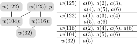
Example 5 (Ex. 4 cont) We get the following answer set:
countAtSets(128) countPW(10) root(w(32)) countWorlds(5) forces(w(125),p) succ(w(32),w(104)) succ(w(32),w(116)) succ(w(104),w(122)) succ(w(104),w(125)) succ(w(116),w(125)) OPTIMUM FOUND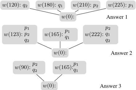
It corresponds to the minimal countermodel displayed in Fig. 3 (isomorphic to the one in Fig. 2). In the table we list the atoms contained in each world; the atom a(6), encoding the goal formula T, does not belong to the root w(32). ✸
Example 6 Let D4 be the goal formula in Fig. 4, having 8 atomic subformulas. We have 49 p-worlds out of 28 = 256 subsets of At(D4). The generator computes three answer sets, corresponding to the models in Fig. 4. The first solution (Answer 1) has 5 worlds and it is not optimal. Then, the solver finds a solution with 4 worlds (Answer 2), finally an answer with 3 worlds (Answer 3), which is optimal. ✸
The previous example shows that in general a minimal countermodel for G cannot be obtained by shrinking a given countermodel for G. Indeed, the minimal countermodels for the formula D4 in Fig. 4 are isomorphic to the bottom model: there is a root, not forcing any propositional variable, and two maximal worlds (w.r.t. ≤), each of them forcing exactly two propositional variables. The top model K1 in Fig. 4 has four maximal worlds, each of them forcing one variable. Using the standard filtration techniques [Chagrov and Zakharyaschev, 1997], there is no way to overlap or delete some of the maximal worlds in K1 and get a 3-world countermodel for D4 (the solver had to discard the maximal worlds chosen to build K1 and to select new ones). Standard proof-search procedures, such as the ones mentioned in the Introduction, build countermodels isomorphic to or bigger than K1; indeed, to falsify D4, at least four distinct maximal worlds are generated, one for each disjunct of D4. Moreover, the computed maximal worlds have in general a "maximal forcing" (either exactly 3 variables or exactly 1 variable are forced), not matching the intermediate circumstance here required (exactly 2 variables are forced). We have tested two provers designed to reduce redundancies in proof-search, and both fail to build a minimal countermodel for D4: STRIP [Larchey-Wendling et al., 2001], based on structural sharing, yields a countermodel having 6 worlds (4 of which are maximal), the prover presented in [Fiorentini and Ferrari, 2017], implementing a forward proof-search strategy, outputs a 5-world countermodel isomorphic to K1.
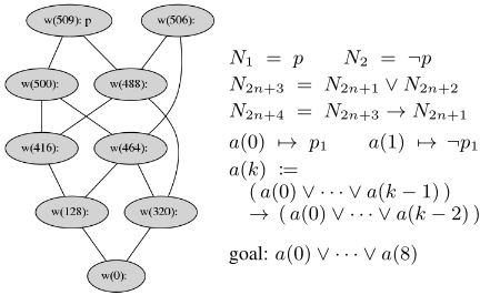
Example 7 Let us consider the one-variable formulas Ni of the Nishimura family [Chagrov and Zakharyaschev, 1997] defined in Fig. 5, which are not valid in IPL. For N17, having 9 atomic subformulas, we have 29 = 512 subsets of At(N17) and only 10 p-worlds. The first answer corresponds to the countermodel in Fig. 5, which is isomorphic to the standard "tower-like" minimal countermodel for N17. ✸
We have also performed some experiments on the nonvalid formulas of Intuitionistic Logic Theorem Proving (ILTP) Library [Raths et al., 2007]. For each tested formula G, Table 1 reports the number of atomic subformulas, the number of p-worlds, the optimum (size of the minimal countermodel) and the CPU time required to compute it 3 . In all the cases, the number of p-worlds is considerably smaller than the number of subsets of At(G): if we worked on all the subsets of At(G), instead of restricting ourselves to pworlds, or we used a naive generation algorithm, the computation would not terminate even with these small formulas. For all the formulas, the minimal countermodel has 2 worlds and coincides with the first answer; with bigger instances, there is no answer within 60 secs. The algorithm is very efficient on Nishimura formulas (see Ex. 7); this depends on the fact that the number of p-worlds essentially coincides with the size of the minimal countermodels.
4 Conclusion
We have presented an ASP program to generate minimal countermodels for non-valid formulas in IPL. Our approach is inspired by [Gor´e and Thomson, 2012; Gor´e et al., 2014] with significant differences. Indeed, Gor´e&al. aim at defining an efficient procedure to test the validity of a goal formula G in IPL (which is a PSPACE-complete problem). To this aim, they build a model KG such that G is valid iff KG is not a countermodel for G. Worlds of KG are represented by proper sets of atomic subformulas of G and, to get an efficient implementation, they exploit BDDs (Binary Decision Diagrams). Here, we deal with a harder problem, since we focus on minimal countermodels for G (and KG in general is not small).
3 Tests were conducted on a standard machine with a 3.0GHz Intel Core(TM)2 Duo CPU and 3.5GB memory,
| Goal formula G | Subsets of At(G) | p-worlds | Opt. | CPU time (in sec.) |
|---|---|---|---|---|
| SYJ207+1.002 | 32768 | 1280 | 2 | 11.85 |
| SYJ208+2.002 | 8192 | 694 | 2 | 6.85 |
| SYJ209+1.005 | 32768 | 921 | 2 | 11.50 |
| SYJ210+1.004 | 65536 | 776 | 2 | 14.95 |
| SYJ211+1.001 | 32768 | 534 | 2 | 7.21 |
| SYJ212+1.005 | 65536 | 975 | 2 | 15.32 |
Accordingly, we use a different encoding (for instance, ¬ is a primitive connective) and a different generation algorithms (we start from a p-world falsifying G and we saturate it by adding the required witnesses).
The program ΠG is quite general and modular; indeed, it can be immediately extended to deal with propositional super-intuitionistic logics based on Kripke semantics, provided that the frame conditions can be captured by the ASP language. An example is the G¨odel-Dummett logic GD, obtained by adding to IPL the axiom schema (A → B)∨(B → A) and semantically characterized by linear frames. We can build countermodels in GD by adding to ΠG the following constraint (lin):
:- world(W1), world(W2), W1 <> W2, not le(W1,W2), not le(W2,W1).This rule forbids the existence of two worlds w1 and w2 such that w1 ̸= w2 and w1 ̸⊂ w2 and w2 ̸⊂ w1. Accordingly, ΠG ∪ {(lin)} is an ASP program to generate minimal countermodels in the logic GD. Other examples of intermediate logics that can be covered by extensions of ΠG are: the logic of bounded depth, the logic of bounded branch, the Here and There logic, closely connected with ASP [Pearce, 1997]. The crucial point is that frame conditions can be freely composed; for instance, if (bd3) encodes the condition "the model has depth at most 3", the program ΠG ∪ {(lin), (bd3)} computes linear countermodels for G having depth at most 3. We remark that standard provers do not enjoy this modularity; in general it is not even obvious how to extend a prover for IPL so as to cover the mentioned logics.
We defer to future work an in-depth classification of the frame conditions that can be expressed in ASP. We also plan to investigate (multi)-modal and temporal logics, also considering other notions of minimality, such as the ones discussed in [Papacchini and Schmidt, 2011; 2014].
Acknowledgments
I am grateful to the reviewers for their valuable suggestions. This work has been partially funded by the INdAM-GNCS project 2018 "Metodi di prova orientati al ragionamento automatico per logiche non-classiche".
@inproceedings{ijcai2019p232,
  title     = {An ASP Approach to Generate Minimal Countermodels in Intuitionistic Propositional Logic},
  author    = {Fiorentini, Camillo},
  booktitle = {Proceedings of the Twenty-Eighth International Joint Conference on
               Artificial Intelligence, {IJCAI-19}},
  publisher = {International Joint Conferences on Artificial Intelligence Organization},
  editor    = {Sarit Kraus},
  pages     = {1675--1681},
  year      = {2019},
  month     = {8},
  note      = {Main track},
  doi       = {10.24963/ijcai.2019/232},
  url       = {https://doi.org/10.24963/ijcai.2019/232},
}
TY - CPAPER TI - An ASP Approach to Generate Minimal Countermodels in Intuitionistic Propositional Logic AU - Fiorentini, Camillo T2 - Proceedings of the Twenty-Eighth International Joint Conference on Artificial Intelligence, IJCAI-19 PB - International Joint Conferences on Artificial Intelligence Organization PY - 2019 SP - 1675 EP - 1681 DO - 10.24963/ijcai.2019/232 UR - https://doi.org/10.24963/ijcai.2019/232 ER -Copied
Machine-readable versions of this paper, for tools and AI agents:





