
SlateQ: A Tractable Decomposition for Reinforcement Learning with Recommendation Sets
Proceedings of the Twenty-Eighth International Joint Conference on Artificial Intelligence. Main track. Pages 2592-2599.
https://doi.org/10.24963/ijcai.2019/360
Keywords
- Machine Learning Applications: Applications of Reinforcement Learning
- Machine Learning: Recommender Systems
- Machine Learning: Reinforcement Learning
Abstract
Reinforcement learning methods for recommender systems optimize recommendations for long-term user engagement. However, since users are often presented with slates of multiple items---which may have interacting effects on user choice---methods are required to deal with the combinatorics of the RL action space. We develop SlateQ, a decomposition of value-based temporal-difference and Q-learning that renders RL tractable with slates. Under mild assumptions on user choice behavior, we show that the long-term value (LTV) of a slate can be decomposed into a tractable function of its component item-wise LTVs. We demonstrate our methods in simulation, and validate the scalability and effectiveness of decomposed TD-learning on YouTube.
- [Abadi et al., 2015] M. Abadi, A. Agarwal, et al. Tensor- Flow: Large-scale machine learning on heterogeneous sys- tems, 2015. Software available from tensorflow.org.
- [Breese et al., 1998] J. Breese, D. Heckerman, and C. Kadie. Empirical analysis of predictive algorithms for collabora- tive filtering. UAI-98, 43-52, Madison, WI, 1998.
- [Charnes and Cooper, 1962] A. Charnes and W. Cooper. Programming with linear fractional functionals. Naval Res. Log. Qrt., 9(3-4):181-186, 1962.
- [Chen and Hausman, 2000] K. Chen and W. Hausman. Mathematical properties of the optimal product line selec- tion problem using choice-based conjoint analysis. Mgmt. Sci., 46(2):327-332, 2000.
- [Chen et al., 2019] M. Chen, A. Beutel, P. Covington, S. Jain, F. Belletti, E. Chi. Top-k off-policy correction for a REINFORCE recommender system. WSDM-19, 456-464.
- [Cheng et al., 2016] H. Cheng, L. Koc, et al. Wide & deep learning for recommender systems. Deep Learn. for Rec. Sys. Workshop, 7-10, Boston, 2016.
- [Choi et al., 2018] S. Choi, H. Ha, U. Hwang, C. Kim, J. Ha, and S. Yoon. Reinforcement learning-based recommender system using biclustering technique. arXiv:1801.05532 [cs.IR], 2018.
- [Covington et al., 2016] P. Covington, J. Adams, and E. Sar- gin. Deep neural networks for YouTube recommendations. RecSys-16, 191-198, Boston, 2016.
- [Deshpande and Karypis, 2004] M. Deshpande and G. Karypis. Item-based top-n recommendation algorithms. ACM TOIS, 22(1):143-177, 2004.
- [Gauci et al., 2018] J. Gauci, E. Conti, et al. Horizon: Face- book's open source applied reinforcement learning plat- form. arXiv:1811.00260 [cs.LG], 2018.
- [Ie et al., 2019] E. Ie, V. Jain, J. Wang, S. Navrekar, R. Agar- wal, R. Wu, H.-Tze Cheng, M. Lustman, V. Gatto, P. Cov- ington, J. McFadden, T. Chandra, and C. Boutilier. Re- inforcement learning for slate-based recommender sys- tems: A tractable decomposition and practical methodol- ogy. arXiv:1905.12767, 2019.
- [Jiang et al., 2019] R. Jiang, S. Gowal, T. Mann, and D. Rezende. Beyond greedy ranking: Slate optimization via list-CVAE. ICLR-19, New Orleans, 2019.
- [Joachims, 2002] T. Joachims. Optimizing search engines using clickthrough data. KDD-02, 133-142, 2002.
- [Konstan et al., 1997] J. Konstan, B. Miller, D. Maltz, J. Her- locker, L. Gordon, J. Riedl. GroupLens: Applying collab- orative filtering to Usenet news. CACM, 40:77-87, 1997.
- [Le and Lauw, 2017] D. Le and H. Lauw. Indexable Bayesian personalized ranking for efficient top-k recom- mendation. CIKM-17, 1389-1398, 2017.
- [Louviere et al., 2000] J. Louviere, D. Hensher, and J. Swait. Stated Choice Methods: Analysis and Application. Cam- bridge Univ. Press, 2000.
- [Metz et al., 2017] L. Metz, J. Ibarz, N. Jaitly, and J. David- son. Discrete sequential prediction of continuous actions for deep RL. arXiv:1705.05035 [cs.LG], 2017.
- [Nemhauser et al., 1978] G. Nemhauser, L. Wolsey, and M. Fisher. An analysis of approximations for maximizing submodular set functions. Math. Prog., 14:265-294, 1978.
- [Puterman, 1994] M. Puterman. Markov Decision Pro- cesses: Discrete Stochastic Dynamic Programming. 1994.
- [Rendle et al., 2010] S. Rendle, C. Freudenthaler, L. Schmidt-Thieme. Factorizing personalized Markov chains for next-basket recommendation. WWW10, 811-820.
- [Salakhutdinov and Mnih, 2007] R. Salakhutdinov and A. Mnih. Probabilistic matrix factorization. NIPS-07, 1257- 1264, Vancouver, 2007.
- [Schön, 2010] C. Schön. On the optimal product line se- lection problem with price discrimination. Mgmt. Sci., 56(5):896-902, 2010.
- [Shani et al., 2005] G. Shani, D. Heckerman, and R. Braf- man. An MDP-based recommender system. JMLR, 6:1265-1295, 2005.
- [Sunehag et al., 2015] P. Sunehag, R. Evans, G. Dulac- Arnold, Y. Zwols, D. Visentin, and B. Coppin. Deep re- inforcement learning with attention for slate Markov de- cision processes with high-dimensional states and actions. arXiv:1512.01124 [cs.AI], 2015.
- [Sutton and Barto, 1998] R. Sutton, A. Barto. Reinforcement Learning: An Introduction. MIT Press, 1998.
- [Swaminathan et al., 2017] A. Swaminathan, A. Krishna- murthy, A. Agarwal, M. Dudik, J. Langford, D. Jose, and I. Zitouni. Off-policy evaluation for slate recommendation. NIPS-17, 3632-3642, Long Beach, CA, 2017.
- [Taghipour et al., 2007] N. Taghipour, A. Kardan, S. Ghidary. Usage-based web recommendations: A reinforcement learning approach. RecSys-07, 113-120.
- [van den Oord et al., 2013] A. van den Oord, S. Dieleman, and B. Schrauwen. Deep content-based music recommen- dation. NIPS-13, 2643-2651, Lake Tahoe, NV, 2013.
- [Van Seijen et al., 2009] H. Van Seijen, H. Van Hasselt, S. Whiteson, and M. Wiering. A theoretical and empirical analysis of expected SARSA. IEEE Symp. Adap. Dyn. Prog. and RL, 177-184, 2009.
- [Viappiani & Boutilier, 2010] P. Viappiani, C. Boutilier. Op- timal Bayesian recommendation sets and myopically opti- mal choice query sets. NIPS, 2352-2360, 2010.
- [Wu et al., 2017] C. Wu, A. Ahmed, A. Beutel, A. Smola, and H. Jing. Recurrent recommender networks. WSDM- 17, 495-503, Cambridge, UK, 2017.
- [Zhao et al., 2018] X. Zhao, L. Xia, L. Zhang, Z. Ding, D. Yin, J. Tang. Deep reinforcement learning for page-wise recommendations. RecSys-18, 95-103, Vancouver, 2018.
References were extracted automatically from the PDF and may contain errors.
Full text extracted automatically from the PDF; figures, tables and equations may differ. The PDF is the version of record.
1 Introduction
Practical recommender systems largely focus on myopic prediction-estimating a user's immediate response to a recommendation-without considering the long-term impact on subsequent user behavior. This can be limiting: modeling a recommendation's stochastic impact on the future affords opportunities to trade off user engagement in the near-term for longer-term benefit (e.g., by probing a user's interests, or improving satisfaction). As a result, recommender systems research has increasingly turned to the sequential nature of user behavior using temporal models, such as hidden Markov models and recurrent neural networks [Rendle et al., 2010; Wu et al., 2017], and long-term planning using reinforcement learning (RL) techniques (e.g., [Gauci et al., 2018; Choi et al., 2018; Zhao et al., 2018]). However, RL for recommendation has largely been confined to restricted domains due to the complexities of deploying such models at scale.
One challenge in many recommenders is that multiple items are recommended to a user simultaneously, sometimes called a recommendation slate. This induces an RL problem with a large combinatorial action space. Recent approaches to RL with such combinatorial actions [Sunehag et al., 2015; Metz et al., 2017] make inroads into this problem, but are unable to scale to problems of the size encountered in large, real-world recommenders, in part because of their generality. In this work, we develop a new slate decomposition technique called SLATEQ that estimates the long-term value (LTV) of a slate of items by directly using the estimated LTV of the individual items on the slate. This decomposition takes advantage of the specifics of user choice behavior, but makes minimal assumptions about user choice.
∗Contact Authors
†Authors Contributed Equally
‡Work done while at Google LLC
Specifically, we first show how the SLATEQ decomposition can be incorporated into temporal difference (TD) learning algorithms, such as SARSA and Q-learning, so that LTVs can be learned at the level of individual items despite the fact that items are always presented to users in slates. This is critical for both generalization and exploration efficiency. We then turn to optimization, i.e., constructing slates that maximize LTV, a required component of policy improvement (e.g., in Q-learning) at training time, and for selecting optimal slates at serving time. Despite the combinatorial (and fractional) nature of the underlying optimization problem, we show that it can be solved in polynomial-time by a two-step reduction to a linear program (LP). We also show that simple top-k and greedy approximations, while having no theoretical guarantees, work well in practice.
Finally, we demonstrate our approach with both offline simulation experiments and an online live experiment on the YouTube video recommendation system. We show that our techniques are scalable and offer significant improvements in user engagement over myopic recommendations. The live experiment also demonstrates how our methodology supports the relatively straightforward deployment of TD and RL methods that build on the learning infrastructure of extant myopic systems. Further details can be found in an expanded, related article [Ie et al., 2019].
2 RelatedWork
Recommender systems have typically relied on collaborative filtering (CF) techniques [Konstan et al., 1997; Breese et al., 1998; Salakhutdinov and Mnih, 2007]. These exploit user feedback on a subset of items (either explicit, e.g., ratings, or implicit, e.g., consumption) to directly estimate user preferences for unseen items. Increasingly, recommenders have moved beyond explicit preference prediction to capture more nuanced aspects of user behavior, for instance, how they respond to specific recommendations, such as pCTR (predicted click-through rate), degree of engagement (e.g., dwell/watch/listen time), ratings, social behavior (e.g., comments, sharing), etc. [van den Oord et al., 2013; Covington et al., 2016; Cheng et al., 2016].
Early attempts to formulate recommendation as an RL problem include an MDP model for shopping recommendation [Shani et al., 2005] and Q-learning for page navigation [Taghipour et al., 2007]), but were limited to very small-scale settings (100s of items, few thousands of users). More recently, biclustering has been combined with RL algorithms [Choi et al., 2018], while several commercial applications are reported in [Gauci et al., 2018; Chen et al., 2019], the latter developing a scalable, off-policy policy-gradient approach (though it does not compute explict LTVs or model slate effects). Zhao et al. [2018] consider actor-critic-based RL in slate recommendation, tested in simulation on an e-commerce data set. While similar in motivation to our approach, it does not explicitly address action-space combinatorics.
Accounting for slates in recommenders is common [Deshpande and Karypis, 2004; Viappiani & Boutilier, 2010; Le and Lauw, 2017] and introduces interesting modeling questions and computational issues due to the combinatorics of slates themselves. Swaminathan et al. [2017] develop offpolicy evaluation and optimization with inverse propensity scores for slate interactions, while Jiang et al. [2019] use of VAEs to model the item distribution and generate slates.
Optimal recommendation slates generally depend on user choice behavior. Choice modeling is widely studied in econometrics, psychology, statistics, operations research and marketing. Probably the most common models of user choice are the multinomial logit (MNL) model and its extensions such as the conditional logit (CL) model [Louviere et al., 2000]. The MNL and CL models are instances of a more general conditional choice format we use below, in which a user i selects item j ∈ A with unnormalized probability v(xij), where v is some function of a user-item feature vector xij :
In the case of CL, v(xij) = eτu(xij) , where u is a utility function. Such models are used to capture consumer choice or other user behavior in various domains. Cascade models [Joachims, 2002] have proven popular as a means of explaining user browsing behavior through (ordered) lists of recommendations, search results, etc., and are especially effective at capturing positional bias.
Designing tractable RL approaches for combinatorial actions-of which slate recommendations are an example-is itself quite challenging. Sequential DQN [Metz et al., 2017] decomposes k-dimensional actions into a sequence of atomic actions, but trades off the exponential size of the action space with a corresponding exponential increase in the size of the state space. Slate MDPs [Sunehag et al., 2015] model slates of primitive actions, and use DQN to learn the value of item slates, and a greedy procedure to construct slates. However, these approaches either require that primitive actions can be executed in isolation (which is not feasible in slate recommenders), or that one maintains an explicit Q-function over slates (hence, failing to address the combinatorics of representation, exploration and generalization).
3 AnMDPModel for Slate Recommendation
In this section, we develop a Markov decision process (MDP) model for content recommendation with slates. We consider a recommender charged with presenting a slate to a user, from which the user selects zero or more items for consumption (e.g., listening to selected music tracks). Once items are consumed, the user can return for additional slate recommendations or terminate the session. The user's response to an item may have multiple dimensions, e.g., degree of engagement (such as consumption time), quality of that engagement, subsequent engagement beyond the recommender's direct control, rating feedback, sharing behavior, etc. We treat degree of engagement as the reward without loss of generality.
Session optimization can be modeled as a MDP with states S, actions A, reward function R and transition kernel P , with discount factor γ. The key components are:
- (i) States S reflect user state, capturing both (relatively static) user features (e.g., demographics, interests) and relevant user history or past behavior (e.g., past recommendations, items consumed, degree of engagement).
- (ii) Actions A are possible recommendation slates. We assume a fixed catalog of items I, so actions are subsets A ⊆ I s.t. |A| = k, where k is the slate size.
- (iii) Transition probability P(s′ |s, A) reflects the probability of the state becoming s′ when action A is taken at s.
- (iv) Reward R(s, A) is the expected reward of a slate, which measures the expected degree of user engagement with items on slate A.
A (stationary, deterministic) policy π : S → A dictates the action to be taken at any state. Its value function V π and action-value (or Q-) function, Qπ are given by:
The optimal policy π∗ maximizes expected value V (s) uniformly over S, and its value-the optimal value function V ∗-is given by the fixed point of the Bellman equation:
The optimal policy satisfies π∗ (s) = arg maxA∈A Q∗ (s, A).
When transition and reward models are provided, optimal policies and value functions can be computed using a variety of methods [Puterman, 1994], though generally these require approximation in large state/action problems. With sampled data, RL methods such as TD-learning SARSA and Q-learning can be used (see Sutton & Barto [1998] for an overview). Given observed transitions and rewards as training data of the form (s, A, r, s′ , A′ ), the Q-function is updated as one of (where α(t) is a learning rate):
SARSA, Eq. (6), is on-policy and estimates the value of the data generating policy π, i.e., the TD-prediction problem on state-action pairs. 1 However, if the policy has sufficient exploration or other forms of stochasticity (as is common in large recommenders), acting greedily w.r.t. Qπ , and using the data so-generated to train a new Q-function, will implement a policy improvement step, and with repetition will converge to the optimal Q-function. Q-learning, Eq. (7), is off-policy and directly estimates the optimal Q-function. Unlike SARSA, Qlearning requires that one compute optimal slates A′ at training time, not just at serving time.
4 SLATEQ: Slate Decomposition for RL
One key challenge in the formulation above is the combinatorial nature of the action space, consisting of all (|I| k ) · k! (ordered) k-sets over I. This poses two difficulties for RL. First, the sheer size of the action space makes sufficient exploration impractical; and generalization of Q-values across slates is challenging without some compressed representation. Second, is the combinatorial optimization problem of finding a slate with maximum Q-value. Without structural assumptions or approximations, this problem cannot meet the real-time latency requirements of production recommender systems (often on the order of tens of milliseconds).
We make two assumptions about the interplay between system dynamics and user choice behavior to develop SLATEQ, a model that allows the Q-value of a slate to be decomposed into a combination of the item-wise Q-values of its constituent items. We first develop the decomposition itself, then show how it can make slate optimization tractable.
4.1 Slate Decomposition of Q-values
We treat selection of no item from the slate as the selection of the null item ⊥, which is an (implicit) item on every slate. We first specify two assumptions about user choice behavior of items from slates that allow the SLATEQ decomposition.
- Single choice (SC): A user consumes a single item from each slate (which may be the null item ⊥).
- Reward/transition dependence on selection (RTDS): The realized reward (user engagement) R(s,A) depends (perhaps stochastically) only on the item i ∈ A consumed by the user. Similarly, the state transition P (s′ |s, A) depends only on the consumed i ∈ A.
1 SARSA is often used to refer to the on-policy control method that includes making policy improvement steps. We use it simply to refer to the TD-method based on SARSA updates as in Eq. (6).
Assumption SC implies that users select only singletons B ⊆ A where |B| = 1. This hold in the conditional choice (including CL) and cascade models described in Sec. 2. While limiting in some settings, in our application (see Sec. 6), users consume one content item at a time. Returning to the slate for a second item is a separate event (with a new state). 2 The RTDS assumption is realistic in many recommenders, especially w.r.t. immediate reward. The transition assumption holds in recommenders where it is a user's direct interaction with items that drives user utility, overall satisfaction, new interests, etc. But it may be treated as a simplifying assumption in other recommenders where unconsumed slate impressions themselves create, say, future curiosity. RTDS allows us to express rewards and state transitions as follows:
Our decomposition of (on-policy) Q-functions for a fixed data-generating policy π relies on an item-wise auxiliary function Qπ (s, i), which represents the LTV of a user consuming an item i, i.e., the LTV of i conditional on it being clicked/selected. Under RTDS, this function is independent of the slate A from which i was selected. We define:
We immediately have, using SC:
Proposition 1. Qπ (s, A) = ∑i∈A P (i|s, A)Qπ (s, i). Proof.
Here Eq. (12) follows immediately from SC and RTDS and Eq. (13) follows from the definition of Qπ .
This simple result gives a complete decomposition of slate Q-values into Q-values for individual items. Hence, the combinatorial challenges disappear if we can learn Qπ (s, i) using TD methods. Fortunately, a simple Q-update fits the bill.
2 Our decomposition can be extended readily to accurately model user selection of multiple items by assuming conditional independence of item-choice probabilities given A.
Given a consumed item i at s with observed reward r, a transition to s′ , and next slate π(s′ ) = A′ , we update Qπ as:
Notice that this update assumes knowledge of the user choice model P(i|s, A). Models such as MNL, CL, and cascade are easily learned from user response data, independent of LTV. Indeed, most recommenders use models that predict clickthrough rates (CTR) for items while ignoring slate interactions. We can use the scores or logits of an existing pCTR model, v, as a proxy for relative appeal of items to the user in state s in any of our models.
Our decomposed SLATEQ update facilitates more compact Q-value models, using items as action inputs rather than slates. This in turn allows for greater generalization and data efficiency. Critically, while SLATEQ learns item-level Qvalues, it can be shown to converge to the correct slate Qvalues under standard assumptions:
Proposition 2. Under standard assumptions on learning rate schedules and exploring starts [Sutton and Barto, 1998], and the assumptions on user choice probabilities, state transitions, and rewards stated in the text above, SLATEQ-using update (14) and definition of slate value (13)-will converge to the true slate Q-function Qπ (s, A) and support greedy policy improvement of π.
Proof. (Brief sketch.) Standard proofs of convergence for TD(0) apply directly for Qπ , except for the introduction of the direct expectation over user choices, i.e., ∑j∈A′ P(j|s′ ,A′ ), rather than samples. But the explicit expectation does not impact convergence (see, e.g., analysis of expected SARSA [Van Seijen et al., 2009]). W.r.t. exploration, if the choice model allows some item j to have P (j|s, A) = 0 for any slate A with π(s) > 0 in some state s, item j at s won't be sampled under π (this is problematic for learning Qπ , not estimating V π ). Thus exploration must account for the choice model (e.g., by sampling all slates, or by configuring exploratory slates that ensure each j is sampled). For most choice models, all items have non-zero choice probability, so standard action-level exploration conditions apply.
Modifying Eq. (10) to obtain Q(s, i)-the optimal (offpolicy) conditional-on-click item-wise Q-function-requires only the replacement of V π (s′ ) with V ∗ (s′ ). Likewise, extending the decomposed update Eq. (14) to full Q-learning needs only to introduce the usual maximization:
Analogs of Props. 1 and 2 easily extend to this case.
4.2 Slate Optimization of Q-values
We now address the combinatorial LTV slate optimization problem, i.e., finding a slate with maximum expected Q-value from A, the space of all (|I| k ) · k! possible (ordered) k-sets over I, given a specific choice model. This is required during training with Q-learning, and serving time when executing the induced greedy policy w.r.t. any Q-function (including when engaging in policy improvement with SARSA). Here we focus on the general conditional choice model (Eq. (1), of which CL and MNL are special cases). In this model, the ordering of items in a slate does not impact choice probabilities, so the action space consists of (|I| k ) (unordered) k-sets.
Exact Optimization
We formulate the LTV slate optimization problem as follows:
Under general conditional choice Eq. (1), including MNL and CL, we can express this as a fractional mixed-integer program (MIP), with binary variables xi ∈ {0, 1} for each item i ∈ I indicating whether i occurs in slate A:
This is a simplified variant of a classic product-line (or assortment) optimization problem [Chen and Hausman, 2000; Sch¨on, 2010]. It can be shown that the binary indicators can be relaxed (see, e.g., Chen & Hausman [2000]) to obtain the following fractional linear program (LP):
The constraint matrix in this relaxed problem is totally unimodular, so the optimal solution is integral and standard nonlinear optimization methods can be used. However, since it is a fractional LP, it is directly amenable to the Charnes-Cooper [1962] transformation and can be recast directly as a (nonfractional) LP. To do so, we introduce an additional variable t that (implicitly) represents the (inverse) choice weight of the selected items t = (v(s,⊥) + ∑j xjv(s, j))-1 , and auxiliary variables yi that represent the products xi · (v(s,⊥) + ∑j xjv(s, j))-1 , giving the following LP:
The optimal solution (y∗ , t∗ ) to this LP yields the optimal xi assignment in the fractional LP Eq. (19) via xi = y∗ i /t∗ . This in turn gives the optimal slate in the original fractional MIP Eq. (17): item i is on the slate if y∗ i > 0. Hence:
Observation 3. LTV slate optimization, Eq. (16), under the general conditional choice model, Eq. (1), and fixed slate size k, is solvable in polynomial-time in the number of items |I|.
Thus full Q-learning with slates using the SLATEQ decomposition imposes at most a small polytime overhead relative to item-wise Q-learning despite its combinatorial nature. Moreover, production systems typically restrict the items to be ranked using a separate retrieval policy, so the set of items in the LP is usually much smaller than the complete set I.
Top-k and Greedy Optimization
While the exact maximization of slates under the conditional choice model can be accomplished in polytime using Q and the item-score function v, we may wish to avoid solving an LP at serving time. A natural heuristic for constructing a slate is to simply add the k items with the highest score: in this case, we insert items into the slate in decreasing order of their "unnormalized expected LTV" v(s, i)Q(s, i). We call this top-k optimization. This incurs only an O(log(I)) overhead relative to the O(I) time required for maximization with item-wise Q-learning.
Top-k is limited since, when considering the item to add to the Lth slot (for 1 < L ≤ k), item scores are not updated to reflect the previous L - 1 items already added to the slate. Greedy optimization, instead of scoring each item ab initio, updates item scores w.r.t. the current partial slate. Specifically, given A′ = {i(1), . . . i(L-1)} of size L - 1 < k, the Lth item is that with maximum marginal value:
We compare top-k and greedy optimizations with the LP solution in our offline simulation experiments below.
Under general conditional choice, neither top-k nor greedy find the optimal slate, per the following counterexample:
| Item | Score (v(s, i)) | Q-value |
| Null | 1 | 0 |
| a | 2 | 0.8 |
| b1, b2 | 1 | 1 |
The null item is always on the slate. Items b1, b2 are identical w.r.t. their behavior. We have V ({a}) = 1.6/3, greater than V ({bi}) = 1/2. Both top-k and greedy will place a on the slate first. However, V ({a, bi}) = 2.6/4, whereas the optimal slate {b1, b2} is valued at 2/3. So for slate size k = 2, neither top-k nor greedy find the optimal slate.
It is not hard to show that the expected value of a slate, viewed as a set function, is neither submodular nor monotone, which prevents the application of standard analyses of greedy algorithms [Nemhauser et al., 1978]. Moreover, top-k can perform arbitrarily poorly in general:
Observation 4. The approximation ratio of the top-k algorithm for slate construction is unbounded.
The following example demonstrates this:
| Item | Score (v(s, i)) | Q-value |
|---|---|---|
| ⊥ | ε | 0 |
| a | ε | 1 |
| b | 1 | ε |
Suppose we have k = 1. Top-k scores item b higher than a, creating the slate with value V ({b}) = ε/(1 + ε), while the optimal slate has value V ({a}) = 1/2.
Algorithm Variants
With multiple slate optimization methods at our disposal, many variants of our RL algorithms exist depending on the optimization method used during training and serving. Given a trained SLATEQ model, we can apply that model to serve users using either top-k, greedy or the LP-based optimal method to generate recommended slates. Below we use the designations TS, GS, or OS to denote these serving protocols, respectively. These designations apply equally to (offpolicy) Q-learned models, (on-policy) SARSA models, and even (non-RL) myopic models. 3
During Q-learning, slate optimization is also required at training time to compute the maximum successor-state Qvalue (Eq. 15). This can also use either of the three optimization methods, which we designate by TT, GT, and OT, respectively. This designation is not applicable when training a myopic model or SARSA (since it is on-policy). Thus for example, QL-OT-OS (resp., QL-OT-TS) refers to Q-learning with optimal training and optimal (resp., top-k) serving, while MYOP-GS refers to myopic recommendation with greedy serving. In our experiments we consider two other baselines: Random, which recommends random slates from the feasible set; and full-slate Q-learning (FSQ), which is a standard, nondecomposed Q-learning method that treats each slate atomically (i.e., holistically) as a single action. The latter is a useful baseline to test whether the SLATEQ decomposition provides leverage for generalization and exploration.
Other Choice Models
SLATEQ is not limited to the choice models (e.g., CL) used above; but the optimization problem varies with the specific model. We discuss additional models (e.g., cascade) in the expanded paper [Ie et al., 2019].
5 Empirical Evaluation: Simulation
We assess the SLATEQ decomposition in a large-scale, live traffic experiment in Sec. 6. In this section we evaluate the quality of SLATEQ on simulated problems using some of the algorithms above. We construct a simulation environment since most public datasets are point-wise, static, and not designed for evaluating multi-step user-recommender interactions. Simulation to evaluate RL is useful even when live experiments are viable, since live evaluation is expensive and can introduce uncontrollable confounding effects.
The simulated environment works as follows (please see the expanded, related article [Ie et al., 2019] for a more detailed description). We have a set of documents D representing content items to be recommended, each reflecting a mixture of topics T . Each d ∈ D is a topic vector d ∈ [0, 1]|T | ; in our experiments, each d has only a single topic T(d). Documents are drawn from distribution PD. Documents also have an (unobservable) inherent quality Ld, drawn randomly from N(µT(d), σ2 ), where µt is a topic-specific mean quality for any t ∈ T (hence topics vary in average quality). Users u ∈ U are characterized in part by their interests in topics, ranging from -1 (completely uninterested) to 1 (fully interested), hence are represented by u ∈ [-1, 1]|T| , drawn from prior PU. User u's interest in document d is given by the dot product I(u, d) = ud.
3 A myopic model is equivalent to a Q-learned model with γ = 0.
At each interaction, m candidate documents are drawn from PD, from which a slate of size k is selected for recommendation. A user chooses one item from the slate using a simple conditional model per Eq. (1): di chosen with probability I(u, di)/ ∑j≤k I(u, dj ). A user's satisfaction S(u, d) with a selected/consumed d is a function f (I(u, d), Ld) of u's interest and d's quality. We use a simple convex combination S(u, d) = αI(u, d) + (1 - α)Ld.
Each u has an initial (unobservable) budget Bu of time to engage with content during a session. Each chosen d reduces u's budget, with a session ending once Bu reaches 0. The budget decreases by a fixed c (which can vary per item if desired) less a bonus that increases with S(u, d); thus, more satisfying items decrease the time remaining in a session at a slower rate. When u consumes d, her interest in topic T(d) is nudged stochastically, biased toward increasing her interest, but with some chance of it decreasing. Thus, this recommender faces a short-term/long-term tradeoff between nudging a user's interests toward topics that tend to have higher quality at the expense of short-term consumption of user budget. Each strategy is evaluated over 5000 simulated users (all results are within a 95% confidence interval).
Myopic vs. Non-myopic Recommendations
We first test the quality of (non-myopic) LTV policies learned using SLATEQ to optimize engagement (γ = 1), using a selection of the SLATEQ algorithms (SARSA vs. Q-learning, different slate optimizations for training/serving). We compare these to myopic scoring (MYOP) (γ = 0), which optimizes only for immediate reward, as well as a Random policy. The following table compares several key metrics:
| Strategy | Avg. Return (%) | Avg. Quality (%) |
|---|---|---|
| Random | 159.2 | -0.5929 |
| MYOP-TS | 166.3 (4.46%) | -0.5428 (8.45%) |
| MYOP-GS | 166.3 (4.46%) | -0.5475 (7.66%) |
| SARSA-TS | 168.4 (5.78%) | -0.4908 (17.22%) |
| SARSA-GS | 172.1 (8.10%) | -0.3876 (34.63%) |
| QL-TT-TS | 168.4 (5.78%) | -0.4931 (16.83%) |
| QL-GT-GS | 172.9 (8.61%) | -0.3772 (36.38%) |
| QL-OT-TS | 169.0 (6.16%) | -0.4905 (17.27%) |
| QL-OT-GS | 173.8 (9.17%) | -0.3408 (42.52%) |
| QL-OT-OS | 174.6 (9.67%) | -0.3056 (48.46%) |
The LTV methods (SARSA and Q-learning) using SLATEQ offer overall improvements in average return per user session (percentage improvements relative to Random are shown in parentheses). For instance, relative to the random baseline, QL-OT-GS provides a 105.6% greater improvement than MYOP-GS. The LTV methods all learn to recommend documents of much higher quality than MYOP. This results in a positive impact on overall session length, which explains the improved return per user. We also see that LP-based slate optimization during training (OT) provides improvements over top-k and greedy optimization (TT, GT) in Qlearning when comparing similar serving regimes (e.g., QL- OT-GS vs. QL-GT-GS, and QL-OT-TS vs. QL-TT-TS). Optimal serving (OS) also shows consistent improvement over top-k and greedy serving-and greedy serving (GS) improves significantly over top-k serving (TS)-when compared under the same training regime. We note that the combination of optimal training and top-k or greedy serving performs well, and is especially useful when serving latency constraints are tight, since optimal training is generally done offline.
Finally, optimizing using Q-learning gives better results than on-policy SARSA (i.e., one-step improvement) under comparable training and serving regimes. But SARSA itself has significantly higher returns than MYOP, demonstrating the value of on-policy RL for recommender systems. Indeed, repeatedly serving-then-training (with some exploration) using SARSA would implement natural, continual policy improvement. These results demonstrate, in this simple synthetic recommender system environment, that using RL to plan long-term interactions can provide significant value in terms of overall engagement.
SLATEQ vs. Holistic Optimization
Next we compare the quality of policies learned using the SLATEQ decomposition to FSQ, the non-decomposed Qlearning method that treats each slate atomically as a single action. We set |T | = 20, m = 10, k = 3 so that we can enumerate all (10 3 ) slates for FSQ maximization. Note that the Qfunction for FSQ requires representation of all (20 3 ) = 1140 slates as actions, which can impede both exploration and generalization. For SLATEQ we test only SARSA-GS. The following table shows our results:
| Avg. Return (%) | Avg. Quality (%) | |
|---|---|---|
| Random | 160.6 | -0.6097 |
| FSQ | 164.2 (2.24%) | -0.5072 (16.81%) |
| SARSA-GS | 170.7 (6.29%) | -0.5340 (12.41%) |
While FSQ, an off-policy Q-learning method, is guaranteed to converge to the optimal slate policy in theory with sufficient exploration, we see that, even when using an onpolicy method like SARSA, SLATEQ methods perform significantly better, offering a 180% greater improvement over Random than FSQ (despite using no additional model iterations for policy improvement). This is due to the fact that FSQ must learn Q-values for 1140 distinct slates, making it difficult to explore and generalize. 4 These results demonstrate the considerable value of the SLATEQ decomposition.
Improved representations could help FSQ generalize better, but the approach is inherently unscalable, while SLATEQ suffers from no such limitations (see Sec. 6). Interestingly, FSQ does converge quickly to a policy that offers recommendations of greater average quality than SLATEQ, but fails to make a suitable tradeoff with user interest.
Robustness to User Choice
We test the robustness of SLATEQ to changes in the choice model. Instead of the assumed choice model above, users select items from the slate using a simple cascade model (e.g., [Joachims, 2002]), where items on the slate are inspected from top-to-bottom with a position-specific probability, and consumed with probability proportional to I(u, d) if SLATEQ continues to outperform MYOP, even when the choice model does not accurately reflect the true environment, demonstrating its relative robustness. SLATEQ can be adapted to other choice models, but since any choice model will be only an approximation of true user behavior, this form of robustness is important.
4 FSQ also takes roughly 6X the training time of SLATEQ over the same number of events.
| Strategy | Avg. Return (%) | Avg. Quality (%) |
|---|---|---|
| Random | 159.9 | -0.5976 |
| MYOP-TS | 163.6 (2.31%) | -0.5100 (14.66%) |
| SARSA-TS | 166.8 (4.32%) | -0.4171 (30.20%) |
| QL-TT-TS | 166.5 (4.13%) | -0.4227 (29.27%) |
| QL-OT-TS | 167.5 (4.75%) | -0.3985 (33.32%) |
| QL-OT-OS | 167.6 (4.82%) | -0.3903 (34.69%) |
Notice that QL-TT and SARSA have inverted relative performance compared to the experiments above. This is due to the fact that Q-learning exploits the (incorrect) choice model to optimize during training, while SARSA, being on-policy, only uses the choice model to compute expectations at serving time. This suggests that on-policy control using SARSA may be more robust than Q-learning in some settings.
6 Empirical Evaluation: Live Experiments
We tested SLATEQ (SARSA-TS specifically) on YouTube with O(109 ) users and O(108 ) items in its corpus. The system is typical of practical recommenders (e.g., [Covington et al., 2016]), with two main components. A candidate generator retrieves a small subset (hundreds) of items from a large corpus that best match a user context. A ranker scores/ranks candidates using a DNN with both user context and item features. It optimizes a combination of several objectives (e.g., clicks, expected engagement, etc.). The extant recommender's policy is myopic, scoring items for the slate using their immediate (predicted) expected engagement.
We replace the myopic engagement measure with an LTV estimate in the ranker's scoring function. We retain other predictions and incorporate them into item scoring as in the myopic model. Our non-myopic recommender maximizes cumulative expected engagement (capped at N days). Since homepage visits can be spaced arbitrarily, we use time-based discounting to handle credit assignment across large time gaps.
Our model extends the myopic ranker to a multi-task feedforward deep network that learns Q(s, i), the predicted longterm engagement of item i (conditional on click) in state s, as well as v(s, i) (for pCTR computation). Our model uses the same state and item features as the myopic model to ensure a reliable comparison. The model is trained using TensorFlow [Abadi et al., 2015] using distributed training and stochastic gradient descent. We train on-policy over pairs of consecutive start page visits, with LTV labels computed using Eq. (14), and use top-k optimization for both training and servingi.e., we test SARSA-TS. The existing myopic recommender (baseline) also builds slates similarly (i.e., MYOP-TS).
We experimented with live traffic for three weeks, treating a small, but statistically significant, fraction of users to recommendations generated by our LTV (SARSA-TS) model.
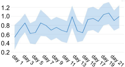
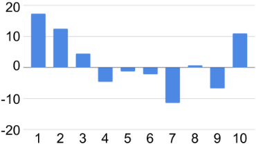
The control is a highly-optimized production machine learning model that optimizes for immediate engagement (MYOPTS). Fig. 1 shows the percentage increase in aggregate user engagement using LTV over the course of the experiment relative to the control, and indicates that our model outperformed the baseline on the key metric under consideration, consistently and significantly. Fig. 2 shows the change in distribution of cumulative engagement originating from items at different positions in the slate. The results show that the users under treatment have more engaging sessions (larger LTVs) from items ranked higher in the slate compared to users in the control group, which suggests that greedy slate optimization performs reasonably in this domain.
7 Conclusion
We have developed SLATEQ, a novel decomposition technique for slate-based RL that allows effective TD and Qlearning using LTV estimates for individual items. Its simple assumptions on user choice-appropriate for many recommender settings-support tractable slate optimization. Our results showed that (i) SLATEQ is robust and scalable (e.g., to large-scale recommenders like YouTube); and (ii) LTV estimation can improve user engagement significantly.
While SLATEQ makes mild assumptions, our methodology can be extended by relaxing these further. Other ongoing directions include: applying SLATEQ to other choice models, further improving scalability, and releasing our simulation environment to the research community.
Acknowledgments
Thanks to Larry Lansing for system optimization and the reviewers for helpful feedback.
@inproceedings{ijcai2019p360,
  title     = {SlateQ: A Tractable Decomposition for Reinforcement Learning with Recommendation Sets},
  author    = {Ie, Eugene and Jain, Vihan and Wang, Jing and Narvekar, Sanmit and Agarwal, Ritesh and Wu, Rui and Cheng, Heng-Tze and Chandra, Tushar and Boutilier, Craig},
  booktitle = {Proceedings of the Twenty-Eighth International Joint Conference on
               Artificial Intelligence, {IJCAI-19}},
  publisher = {International Joint Conferences on Artificial Intelligence Organization},
  editor    = {Sarit Kraus},
  pages     = {2592--2599},
  year      = {2019},
  month     = {8},
  note      = {Main track},
  doi       = {10.24963/ijcai.2019/360},
  url       = {https://doi.org/10.24963/ijcai.2019/360},
}
TY - CPAPER TI - SlateQ: A Tractable Decomposition for Reinforcement Learning with Recommendation Sets AU - Ie, Eugene AU - Jain, Vihan AU - Wang, Jing AU - Narvekar, Sanmit AU - Agarwal, Ritesh AU - Wu, Rui AU - Cheng, Heng-Tze AU - Chandra, Tushar AU - Boutilier, Craig T2 - Proceedings of the Twenty-Eighth International Joint Conference on Artificial Intelligence, IJCAI-19 PB - International Joint Conferences on Artificial Intelligence Organization PY - 2019 SP - 2592 EP - 2599 DO - 10.24963/ijcai.2019/360 UR - https://doi.org/10.24963/ijcai.2019/360 ER -Copied
Machine-readable versions of this paper, for tools and AI agents:





