
MR-GNN: Multi-Resolution and Dual Graph Neural Network for Predicting Structured Entity Interactions
Proceedings of the Twenty-Eighth International Joint Conference on Artificial Intelligence. Main track. Pages 3968-3974.
https://doi.org/10.24963/ijcai.2019/551
Keywords
- Multidisciplinary Topics and Applications: Biology and Medicine
- Machine Learning: Classification
- Machine Learning Applications: Bio;Medicine
- Machine Learning: Deep Learning
Abstract
Predicting interactions between structured entities lies at the core of numerous tasks such as drug regimen and new material design. In recent years, graph neural networks have become attractive. They represent structured entities as graphs, and then extract features from each individual graph using graph convolution operations. However, these methods have some limitations: i) their networks only extract features from a fix-sized subgraph structure (i.e., a fix-sized receptive field) of each node, and ignore features in substructures of different sizes, and ii) features are extracted by considering each entity independently, which may not effectively reflect the interaction between two entities. To resolve these problems, we present {\em MR-GNN}, an end-to-end graph neural network with the following features: i) it uses a multi-resolution based architecture to extract node features from different neighborhoods of each node, and, ii) it uses dual graph-state long short-term memory networks (LSTMs) to summarize local features of each graph and extracts the interaction features between pairwise graphs. Experiments conducted on real-world datasets show that MR-GNN improves the prediction of state-of-the-art methods.
- [Altae-Tran et al., 2017] Han Altae-Tran, Bharath Ramsun- dar, Aneesh S. Pappu, and Vijay Pande. Low data drug discovery with one-shot learning. ACS CENTRAL SCI, 3(4):283-293, 2017.
- [Atwood and Towsley, 2016] James Atwood and Don Towsley. Diffusion-convolutional neural networks. In NIPS, pages 1993-2001, 2016.
- [Bai et al., 2018] Yunsheng Bai, Hao Ding, Song Bian, T- ing Chen, Yizhou Sun, and Wei Wang. Graph edit distance computation via graph neural networks. arX- iv:1808.05689, 2018.
- [Defferrard et al., 2016] Michaël Defferrard, Xavier Bres- son, and Pierre Vandergheynst. Convolutional neural net- works on graphs with fast localized spectral filtering. In NIPS, pages 3844-3852, 2016.
- [Duvenaud et al., 2015] David Duvenaud, Dougal Maclau- rin, Jorge Aguilera-Iparraguirre, Rafael Gómez- Bombarell, Timothy Hirzel, Alán Aspuru-Guzik, and Ryan P. Adams. Convolutional networks on graphs for learning molecular fingerprints. In NIPS, pages 2224-2232, 2015.
- [Fout et al., 2017] Alex Fout, Jonathon Byrd, Basir Shariat, and Asa Ben-Hur. Protein interface prediction using graph convolutional networks. In NIPS, pages 6530-6539, 2017.
- [Hamilton et al., 2017a] Will Hamilton, Zhitao Ying, and Ju- re Leskovec. Inductive representation learning on large graphs. In NIPS, pages 1024-1034, 2017.
- [Hamilton et al., 2017b] William L. Hamilton, Rex Ying, and Jure Leskovec. Representation learning on graphs: Methods and applications. 2017.
- [Henaff et al., 2015] Mikael Henaff, Joan Bruna, and Yann LeCun. Deep convolutional networks on graph-structured data. arXiv:1506.05163, 2015.
- [Kearnes et al., 2016] Steven Kearnes, Kevin Mccloskey, Marc Berndl, Vijay Pande, and Patrick Riley. Molecular graph convolutions: moving beyond fingerprints. J COM- PUT AID MOL DES, 30(8):1-14, 2016.
- [Kipf and Welling, 2017] Thomas N. Kipf and Max Welling. Semi-supervised classification with graph convolutional networks. In ICLR, 2017.
- [Kwon and Yoon, 2017] Sunyoung Kwon and Sungroh Y- oon. Deepcci: End-to-end deep learning for chemical- chemical interaction prediction. arXiv:1704.08432, 2017.
- [Li et al., 2015] Yujia Li, Daniel Tarlow, Marc Brockschmidt, and Richard Zemel. Gated graph se- quence neural networks. arXiv:1511.05493, 2015.
- [Li et al., 2017] Junying Li, Deng Cai, and Xiaofei He. Learning graph-level representation for drug discovery. arXiv:1709.03741, 2017.
- [Perozzi et al., 2014] Bryan Perozzi, Rami Al-Rfou, and Steven Skiena. Deepwalk: Online learning of social rep- resentations. In SIGKDD, pages 701-710, 2014.
- [Ryu et al., 2018] Jae Yong Ryu, Hyun Uk Kim, and Sang Yup Lee. Deep learning improves prediction of drug- drug and drug-food interactions. PNAS, 115(18):E4304, 2018. Sukhbaatar et al., 2016] Sainbayar Sukhbaatar, Rob Fergus, et al. Learning multiagent communication with backprop- agation. In in NIPS, pages 2244-2252, 2016.
- [Tang et al., 2015] Jian Tang, Meng Qu, Mingzhe Wang, Ming Zhang, Jun Yan, and Qiaozhu Mei. Line: Large- scale information network embedding. In WWW, pages 1067-1077, 2015.
- [Tian et al., 2016] Kai Tian, Mingyu Shao, Yang Wang, Ji- hong Guan, and Shuigeng Zhou. Boosting compound- protein interaction prediction by deep learning. Methods, 110:64-72, 2016.
- [Velickovic et al., 2018] Petar Velickovic, Guillem Cucu- rull, Arantxa Casanova, Adriana Romero, Pietro Lio, and Yoshua Bengio. Graph attention networks. arX- iv:1806.03536, 2018.
- [Wang et al., 2016] Daixin Wang, Peng Cui, and Wenwu Zhu. Structural deep network embedding. In SIGKDD, pages 1225-1234, 2016.
- [Weininger, 1988] David Weininger. Smiles, a chemical lan- guage and information system. 1. introduction to method- ology and encoding rules. J. Chem. Inf. Comput. Sci., 28(1):31-36, 1988.
- [Yanardag and Vishwanathan, 2015] Pinar Yanardag and S. V. N. Vishwanathan. Deep graph kernels. In SIGKDD, pages 1365-1374, 2015.
- [Zhang and Chen, 2018] Muhan Zhang and Yixin Chen. Link prediction based on graph neural networks. arX- iv:1802.09691, 2018.
- [Zhang et al., 2018a] Muhan Zhang, Zhicheng Cui, and Y. Neumann, M. & Chen. An end-to-end deep learning architecture for graph classification. In AAAI, 2018.
- [Zhang et al., 2018b] Yuhao Zhang, Peng Qi, and Christo- pher D Manning. Graph convolution over pruned dependency trees improves relation extraction. arX- iv:1809.10185, 2018.
- [Zhao et al., 2018] Xiaohan Zhao, Bo Zong, Ziyu Guan, Kai Zhang, and Wei Zhao. Substructure assembling network for graph classification. AAAI, 2018.
- [Zitnik et al., 2018] Marinka Zitnik, Monica Agrawal, and Jure Leskovec. Modeling polypharmacy side effect- s with graph convolutional networks. Bioinformatics, 34(13):457-466, 2018.
References were extracted automatically from the PDF and may contain errors.
Full text extracted automatically from the PDF; figures, tables and equations may differ. The PDF is the version of record.
1 Introduction
A large variety of applications require understanding the interactions between structured entities. For example, when one medicine is taken together with another, each medicine's intended efficacy may be altered substantially (see Fig. 1). Understanding their interactions is important to minimize the side effects and maximize the synergistic benefits [Ryu et al., 2018]. In chemistry, understanding what chemical reactions will occur between two chemicals is helpful in designing new materials with desired properties [Kwon and Yoon, 2017]. Despite its importance, examining all interactions by performing clinical or laboratory experiments is impractical N H
∗Corresponding Authors
†Nuo Xu and Pinghui Wang contributed equally to this work.
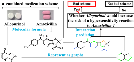
Figure 1: Overview of graph-based framework. We transform two drugs Allopurinol and Amoxicillin into graphs, where nodes represent atoms and edges refer to chemical bonds between atoms, and predict interactions between them. When there exists an adverse reaction between them, they cannot be taken together.
due to the potential harms to patients and also highly time and monetary costs.
Recently, machine learning methods have been proposed to address this problem, and they are demonstrated to be effective in many tasks [Duvenaud et al., 2015; Li et al., 2017; Tian et al., 2016; Ryu et al., 2018]. These methods use features extracted from entities to train a classifier to predict entity interactions. However, features have to be carefully provided by domain experts [Ryu et al., 2018; Tian et al., 2016], and it is labor-intensive. To automate feature extraction, graph convolution neural networks (GCNs) have been proposed [Fout et al., 2017; Kwon and Yoon, 2017; Zitnik et al., 2018]. GCNs represent structured entities as graphs, and use graph convolution operators to extract features. One of the state-of-the-art GCN models, proposed by Alex et al. [2017], extracts features from the 3-hop neighborhood of each node. We thus say that their model uses a fix-sized receptive field (RF). However, using a fix-sized RF to extract features may have limitations, which can be illustrated by the following example.
Example 1. Figure 2 shows two weak acids, i.e., Hydroquinone and Acetic acid. They are weak acids due to the existence of substructures phenolic hydroxyl (ArOH) and carboxyl (COOH), respectively. Representing these two chemical compounds as graphs, we need a three-hop neighborhood to accurately extract ArOH from Hydroquinone, and a twohop neighborhood to accurately extract COOH from Acetic acid. While using a fix-sized neighborhood will result in that either incomplete substructures being extracted (i.e., RF is too small), or useless substructures being included (i.e., RF is too large).
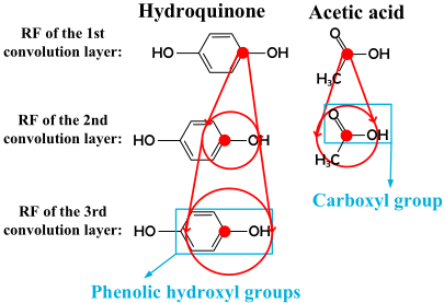
Another limitation of existing GCNs is that, they learn each graph's representation independently, and model the interactions only in the final prediction process. However, for different entities, the interaction also occurs by substructures of different size. Take Fig. 2 for example again, when these two weak acids are neutralized with the same strong base, the interaction can be accurately modeled by features of the second convolution layer for Acetic acid because the key substructure ArOH can be accurately extracted. But for Hydroquinone, the best choice is to model the interaction by features of the third convolution layer. Thus, modeling the interactions only in the final process may make a lot of noise to the prediction.
To address these limitations, this work presents a novel GCN model named Multi-Resolution RF based Graph Neural Network (MR-GNN), which leverages different-sized local features and models interaction during the procedure of feature extraction to predict structured entity interactions.
MR-GNN uses a multi-resolution RF, which consists of multiple graph convolution layers with different RFs, to extract local structure features effectively (see Fig. 2). When aggregating these multi-resolution local features, MR-GNN uses two key dual graph-state LSTMs. One is Summary-LSTM (S-LSTM), which aggregates multi-resolution local features for each graph. Compared with the straightforward method that simply sums all multi-resolution features up, S-LSTM learns additional effective features by modeling the diffusion process of node information in graphs which can greatly enrich the graph representation. The other is Interaction-LSTM (I-LSTM), which extracts interaction features between pairwise graphs during the procedure of feature extraction.
Our contributions are as follows:
- In MR-GNN, we design a multi-resolution based architecture that mines features from multi-scale substructures to predict graph interactions. It is more effective than considering only fix-sized RFs.
- We develop two dual graph-state LSTMs: One summarizes subgraph features of multi-sized RFs while modeling the diffusion process of node information, and the
- other extracts interaction features for pairwise graphs during feature extraction.
- Experimental results on two benchmark datasets show that MR-GNN outperforms the state-of-the-art methods.
2 ProblemDefinition
Notations. We denote a structured entity by a graph G = (V,E), where V is the node set and E is the edge set. Each specific node vi ∈ V is associated with a c-dimension feature vector fi ∈ Rc . The feature vectors can also be lowdimensional latent representations/embeddings for nodes or explicit features which intuitively reflects node attributes. Meanwhile, let Ni ⊆ V denote vi's neighbors, and di ≜ |Ni| denote vi's degree.
Entity Interaction Prediction. Let L ≜ {li|i = 1, 2 . . . , k} denote a set of k interaction labels between two entities. The entity interaction prediction task is formulated as a supervised learning problem: Given training dataset D ≜ {(GX,GY )s, ˆRs}qs=1 where (GX,GY )s is an input entity pair, and ˆRs ∈ L is the corresponding interaction label; let q denote the size of D, we want to accurately predict the interaction label R ∈ L of an unseen entity pair (GX, GY )new.
3 Method
In this section, we propose a graph neural network, i.e., MRGNN, to address the entity interaction prediction problem.
3.1 Overview
Figure 3 depicts the architecture of MR-GNN, which mainly consists of three parts: 1) multiple weighted graph convolution layers, which extract structure features from receptive fields of different sizes, 2) dual graph-state LSTMs, which summarize multi-resolution structure features and extract interaction features, and 3) fully connected layers, which predict the entity interaction labels.
3.2 Weighted Graph Convolution Layers
Before introducing the motivation and design of our weighted graph convolution operators in detail, we elaborate the standard graph convolution operator.
Standard Graph Convolution Operator. Inspired by the convolution operator on images, for a specific node in a graph, the general spatial graph convolution [Duvenaud et al., 2015] aggregates features of a node as well as its one-hop neighbors' as the node's new features. Based on the above definition, take the node vi as an example, the formula is:
where f (t+1) i denotes the feature vector of vi in the (t + 1)th graph convolution layer, W (t) di is the weight matrix associated with the center node vi and σ(·) is the tanh activation function. Note that f (0) i = fi.
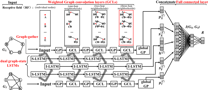
Because the output graph of each graph convolution layer is exactly same as the input graph, MR-GNN can conveniently learn the structural characteristics of different resolutions through different iterations of the graph convolution layer. Take the node A in Fig. 3 as an example, after three iterations of graph convolution layer, the receptive field in the third graph convolution layer is a three-hop neighborhood centered on it.
However, since graphs are not regular grids compared with images, it is difficult for the existing graph convolution operator to distinguish the weight by spatial orientation position like the convolution operator on grid-like data, e.g., in the image processing, the right neighbor and the left neighbor of a pixel can be treated with different weight for each convolution kernel. Inspired by the fact that the degree of nodes can well reflect the importance of nodes in a network for many applications. We modify the graph convolution operator by adding weights according to the node degree di. (Other metrics such as betweenness centrality can also work well. In this paper we choose the degree of nodes because of the simplicity of calculation.) Furthermore, Sukhbaatar et al. [2016] treats different agents with different weights in order to distinguish the feature of the original node and the features of neighboring nodes. We treat each node and its neighbors with different weight matrixes, Φ and Ψ. Our improved weighted graph convolution is as follows:
where Φ(t) di ,Ψ(t) di ∈ Rct×ct+1 denote the weight of node vi with degree di, ct+1 denotes the dimension of the feature vector in the (t+1)th graph convolution layer, and b(t) ∈ R1×ct+1 is a bias. We let c0 = c.
After each convolution operation, similar to the classical CNN, we use a graph pooling operation GP (·) to summarize the information within neighborhoods (i.e., a center node and its neighbors). For a specific node, the Graph Pooling [AltaeTran et al., 2017] returns a new feature vector of which each element is the maximum activation of the corresponding element of one-hop neighborhood at this node. We denote this operation by the following formula and get the feature vectors of the next layer:
3.3 Graph-gather Layers
Graph interaction prediction is a graph-level problem rather than a node-level problem. To learn the graph-level features of different-sized receptive fields, we aggregate the node representations of each convolution layer's graph to a graphstate by a graph-gather layer. Graph-gather layers compute a weighted sum of all node vectors in the connected graph convolution layers. The formula is:
where Θ(t) di ∈ Rct×cG is the graph-gather weight of nodes with di degree in the tth graph convolution layer, g(t) is the graph-state vector of the tth convolution layer, cG denotes the dimension of graph-states, m is the nodes' number in the graph and β(t) di ∈ R1×cG is a bias. Specially, the first graphstate g(0) only includes all individual nodes' information.
3.4 Dual Graph-state Lstms
To solve graph-level tasks, the existing graph convolution networks (GCNs) methods [Altae-Tran et al., 2017] generally choose the graph-state of the last convolution layer, which has the largest receptive fields, as input for subsequent prediction. But such state may loss many important features.
Referring to the CNN on images, there are multiple convolution kernels for extracting different features in each convolution layer, which ensure the hidden representation of the final convolution layer can fully learn features of input images. However, GCN is equivalent to CNN that only has one kernel in each layer. It is difficult for the output of the final graph convolution layer to fully learn all features in the large receptive fields, especially for structure features of small receptive field. The straightforward way is to design multiple graph convolution kernels and aggregate the output of them. However it is computational expensive.
To solve the above problem, we propose a multi-resolution based architecture in our model, in which the graph-state of each graph convolution layer is leveraged to learn the final representation. We propose a Summary-LSMT (S-LSTM) to aggregate the graph-states of different-sized receptive fields for learning the final features comprehensively. Instead of the straightforward method that directly sums all graph-states up, S-LSTM models the node information diffusion process of graphs by sequentially receiving the graph-state g(t) with receptive field from small to large as inputs. It is inspired by the idea a representation that encapsulates graph diffusion can provide a better basis for prediction than the graph itself. The formula of S-LSTM is:
where s(t+1) ∈ R1×cG is the (t +1)th hidden vector of SLSTM. To further enhance the global information of graphs, we concatenate the final hidden output S(f) of S-LSTM and the output p(f) of global graph pooling layer as the final graph-state of the input graph:
where p(f) = GP(f (f) v1 , ..., f (f) vm ) ∈ R1×cf is the result of global graph pooling on the final graph convolution layer.
In addition, to extract the interaction features of pairwise graphs, we propose an Interaction-LSTM (I-LSTM) which takes the concatenation of dual graph-states as input:
where h(t+1) ∈ R1×2cG is the (t +1)th hidden vector of ILSTM .We initialize s(0) and h(0) as an all-zero vector and the S-LSTM is shared to both input graphs.
3.5 Fully Connected Layers
For the interaction prediction, we simply concatenate the final graph representations and interaction features of input graphs (i.e., e(f) X , e(f) Y and h(f) ) and use fully connected layers for prediction. Formally, we have:
where fi(x) = Wix + bi, i = 1, 2, are linear operations, W1 ∈ R(2cf+4cG)×ck and W2 ∈ Rck×k are trainable weight matrices, ck is the dimension of the hidden vector, and k is the number of interaction labels. The activation function σr(·) is a rectified linear unit (ReLU), i.e., σr(x) = max(0, x). R is the output of softmax function σs(·), the j th element of R is computed as rj = erj ∑ki=0 eri . At last, we choose the cross entropy function as loss function, that is:
where ˆR ∈ R1×k is the ground-truth vector.
4 Experiment
In this section, we conduct experiments to validate our method 1 . We consider two prediction tasks: 1) predicting whether there is an interaction between two chemicals (i.e., binary classification), and 2) predicting the interaction label between two drugs (i.e., multi-class classification).
4.1 Dataset
CCI Dataset. For the binary classification task, we use the CCI dataset [Kwon and Yoon, 2017]. This dataset uses a score ranging from 0 to 999 to describe the interaction level between two compounds. The higher the score is, the larger probability the interaction will occur with. According to threshold scores 900, 800 and 700, we got positive samples of three datasets: CCI900, CCI800, and CCI700, which contain 11990, 73602, 114734 graphs, and 19624, 151796, 343277 graph pairs respectively. As for negative samples, we choose the chemical pairs of which the score is 0. For each pair of chemicals, we assign a label "1" or "0" to indicate whether an interaction occurs between them. We use a public available API, DeepChem 2 , to convert compounds to graphs, that each node has a 75-dimension feature vector.
DDI Dataset. For the multi-class classification task, we use the DDI dataset [Ryu et al., 2018], which contains 1704 drug molecule graphs and 191400 graph pairs. This dataset contains 86 interaction labels, and each drug is represented by SMILES string [Weininger, 1988]. In our preprocessing, we remove the data items that cannot be converted into graphs from SMILES strings.
4.2 Baselines
We compare our method with the following state-of-the-art models:
- DeepCCI [Kwon and Yoon, 2017] is one of the stateof-the-art methods on the CCI datasets. It represents SMILES strings of chemicals as one-hot vector matrices and use classical CNN to predict interaction labels.
- DeepDDI [Ryu et al., 2018] is one of the state-of-the-art methods on the DDI dataset. DeepDDI designs a feature called structural similarity profile (SSP) combined with multilayer perceptron (MLP) for prediction.
- PIP [Fout et al., 2017] is proposed to predict the protein interface. It extracts features from the fixed three-hop neighborhood for each node to learn a node representation. In this paper, when building this model, we use our graph-gather layer to aggregate node representations to get the graph representation.
- DGCNN [Zhang et al., 2018a] uses the standard graph convolution operator as described in Section 3. It concatenates the node vectors of each graph convolution layer and applies CNN with a node ordering scheme to generate a graph representation.
1 Code available at https://github.com/prometheusXN/MR-GNN
2 https://deepchem.io/
| CCI900 | CCI800 | CCI700 | ||||||||||
|---|---|---|---|---|---|---|---|---|---|---|---|---|
| AUC | accuracy | recall | F1 | AUC | accuracy | recall | F1 | AUC | accuracy | recall | F1 | |
| PIP | 93.92 | 87.95 | 88.73 | 87.66 | 98.49 | 94.67 | 94.74 | 94.59 | 98.92 | 95.53 | 94.96 | 95.52 |
| SNR | 91.86 | 83.99 | 79.40 | 82.95 | 97.18 | 91.19 | 89.81 | 90.95 | 98.04 | 92.87 | 92.21 | 92.85 |
| DGCNN | 95.14 | 85.53 | 84.72 | 85.12 | 97.13 | 91.54 | 91.55 | 91.43 | 97.95 | 93.13 | 92.65 | 93.13 |
| DeepDDI | 90.30 | 83.74 | 82.94 | 83.58 | 95.43 | 89.73 | 90.10 | 89.88 | 96.48 | 91.77 | 91.74 | 91.80 |
| DeepCCI | 95.14 | 88.11 | 88.90 | 87.95 | 98.69 | 95.38 | 94.93 | 95.34 | 99.22 | 96.25 | 95.54 | 96.25 |
| MR-GNN | 95.67 | 90.16 | 91.21 | 90.05 | 98.76 | 95.44 | 95.28 | 95.38 | 99.25 | 96.51 | 96.08 | 96.51 |
- SNR [Li et al., 2017] uses the similar graph convolution layer as our method. The difference is that this work introduces an additional node that sums all nodes features up to a graph representation.
4.3 Binary Classification
We divide each CCI dataset into a training dataset and a testing dataset with ratio 9 : 1, and randomly choose 1/5 of the training dataset as a validation dataset. We set the three graph convolution layers with 384, 384, 384 output units, respectively. We set 128 output units of graph-gather layers as the same as the LSTM layer. The fully connected layer has 64 hidden units followed by a softmax layer as the output layer. We set the learning rate to 0.0001. To evaluate the experimental results, we choose four metrics: area under ROC curve (AUC), accuracy, recall, and F1.
Table 2 shows the performance of different methods. MRGNN performs the best in terms of all of the evaluation metrics. Compared with the state-of-the-art method DeepCCI, our MR-GNN improves accuracy by 0.6%-2.5%, F1 by 0.6%-2.2%, recall by 1.0%-2.3%, and AUC by 0.05%- 0.32%. As for little improvement of AUC, we think it is ascribed to the fact that the basic value is too large to provide enough space for improvement. When translated into the remaining space, the AUC is increased by 4.2%-11.8%. The performance improvement proves that features extraction of MR-GNN, which represents structured entities as graphs for features extraction, is more effective than DeepCCI, which treats SMILES string as character sequence without considering topological information of structured entities. Compared with PIP, the performance of MR-GNN demonstrates that the multi-resolution based architecture is more effective than the fix-sized RF based framework. In addition, compared with SNR which directly sums all node features to get the graph representation, experimental results prove that our S-LSTM summarizes the local features more effectively and more comprehensively. We attribute this improvement to the diffusion process and the interaction that our graph-state LSTM modeled during the procedure of feature extraction, which is effective for the prediction.
4.4 Multi-class Classification
To make an intuitional comparison, similar to DeepDDI, we use 60%, 20%, 20% of dataset for the training, validation and testing, respectively. All hyper-parameter selections are the same as the binary classification task. To evaluate the experimental results, we choose five metrics on the multiclassification problem: AUPRC, Micro average, Macro recall, Macro precision, and Macro F1. (In particular, we choose the AUPRC metric due to the imbalance of the DDI dataset.) We show the results on DDI dataset in Table 3.
We observe that MR-GNN performs the best in terms of all five evaluation metrics. MR-GNN improves these five metrics by 1.58%, 5.23%, 5.46%, 5.60% and 1.58%, respectively. Compared with the state-of-the-art method DeepDDI, the performance improvement of MR-GNN is attributed to the higher quality representations learned by end-to-end training instead of the human-designed representation called SSP. In addition, we also conduct experiments on CCI and DDI datasets, and we observe that MR-GNN indeed improves performance.
Ablation Experiment. We also conducted ablation experiments on the DDI dataset to study the effects of three components in our model (namely S-LSTM, I-LSTM, and weighted GCL). We find that each of these three components can improve performance. Among them, weighted GCLs contributes most significantly, then comes S-LSTM and I-LSTM.
4.5 Efficiency and Robustness
In the third experiment, we conduct experiments to analyze the efficiency and robustness of MR-GNN.
Effects of TrainingDataset Size. We carried out a comparative experiment with different size of training datasets from 30% to 70% on the CCI900 dataset. In each comparative experiments, we kept the same 10% of the dataset as the test dataset to evaluate the performance of all six methods. Figure 4(a) shows that MR-GNN always performs the best under different training dataset size. In particular, as the training dataset proportions increases, the improvement of MR-GNN increases significantly, demonstrating that our MR-GNN has better robustness. This is due to the fact that MR-GNN is good at learning subgraph information of different-sized receptive fields, especially subgraphs of small receptive fields that often appear in various graphs.
| Mi avg | Ma recall | Ma pre | Ma F1 | AUPRC | |
|---|---|---|---|---|---|
| PIP | 92.73 | 87.45 | 89.47 | 87.88 | 91.60 |
| SNR | 82.91 | 79.88 | 76.71 | 76.88 | 81.85 |
| DGCNN | 86.63 | 72.02 | 79.15 | 74.32 | 85.54 |
| DeepCCI | 87.38 | 79.91 | 88.86 | 82.73 | 86.29 |
| DeepDDI | 92.64 | 83.86 | 89.58 | 85.70 | 91.52 |
| MR-GNN | 94.31 | 92.68 | 94.94 | 93.48 | 93.18 |
| -no I-LSTM | 94.11 | 91.96 | 94.23 | 92.81 | 92.98 |
| -no S-LSTM | 94.05 | 90.31 | 94.53 | 91.82 | 92.92 |
| -no w-GCL | 93.86 | 89.33 | 92.83 | 90.38 | 92.74 |
| -no LSTMs | 92.83 | 86.38 | 91.61 | 88.11 | 91.71 |
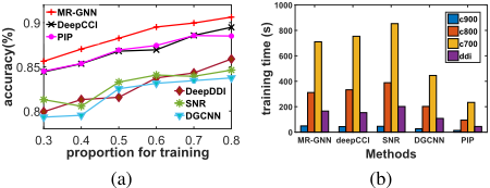
Training Efficiency. Figure 4(b) shows that the training time of MR-GNN is at a moderate level among all methods. Although the graph-state LSTMs takes the additional time, the training of MR-GNN is still fast and acceptable.
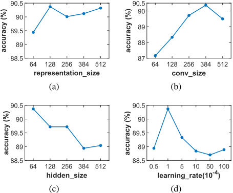
Effects of Hyper-parameter Variation. In this experiment, we consider the impact of hyper-parameters of MRGNN: the output units number of GCLs (conv size) and LSTMs (represent size), the hidden units number of the fully connected layer (hidden size), and learning rate. The results are shown in Fig. 5. We see that the impact of hyper-parameter variation is insignificant (the absolute difference is less than 2%). Fig. 5(a) shows that larger represent size provides a better performance (with an salient point at represent size = 128). Fig. 5(b) shows that similar result of conv size while a salient point is at conv size = 384. The performance increases fast when conv size < 384 and slightly declines when conv size ≥ 384. As for learning rate and hidden size, the best point appears at 1 × 10⁻⁴ and 512, respectively.
5 RelatedWork
Node Based Applications. Many neural network based methods have been proposed to solve the node-level tasks such as node classification [Henaff et al., 2015; Li et al., 2015; Defferrard et al., 2016; Kipf and Welling, 2017; Veli¨ckovic et al., 2018], link prediction [Zhang and Chen, 2018; Zhang et al., 2018b], etc. They rely on node embedding techniques, including skip-gram based methods like DeepWalk [Perozzi et al., 2014] and LINE [Tang et al., 2015], autoencoder based methods like SDNE [Wang et al., 2016], neighbor aggregation based methods like GCN [Defferrard et al., 2016; Kipf and Welling, 2017] and GraphSAGE [Hamilton et al., 2017a], etc.
SingleGraphBasedApplications. Attention also has been paid on the graph-level tasks. Most existing works focus on classifying graphs and predicting graphs' properties [Duvenaud et al., 2015; Atwood and Towsley, 2016; Li et al., 2017; Zhang et al., 2018a] and they compute one embedding per graph. To learn graph representations, the most straightforward way is to aggregate node embeddings, including average-based methods (simple average and weight average) [Li et al., 2017; Duvenaud et al., 2015; Zhao et al., 2018], sum-based methods [Hamilton et al., 2017b] and some more sophisticated schemes, such as aggregating nodes via histograms [Kearnes et al., 2016] or learning node ordering to make graphs suitable for CNN [Zhang et al., 2018a].
Pairwise Graph Based Applications. Nowadays, very little neural network based works pay attention to the pairwise graph based tasks whose input is a pair of graphs. However, most existing works focus on learning "similarity" relation between graphs [Bai et al., 2018; Yanardag and Vishwanathan, 2015] or links between nodes across graphs [Fout et al., 2017]. In this work, we study the prediction of the universal graph interactions.
6 Conclusion
In this paper, we propose a novel graph neural network, i.e., MR-GNN, to predict the interactions between structured entities. MR-GNN can learn comprehensive and effective features by leveraging a multi-resolution architecture. We empirically analyze the performance of MR-GNN on different interaction prediction tasks, and the results demonstrate the effectiveness of our model. Moreover, MR-GNN can easily be extended to large graphs by assigning node weights to node groups that based on the distribution of node degrees. In the future, we will apply it to more other domains.
Acknowledgments
The research presented in this paper is supported in part by National Key R&D Program of China (2018YFC0830500), National Natural Science Foundation of China (UI736205, 61603290), Shenzhen Basic Research Grant (ICYJ20170816100819428), Natural Science Basic Research Plan in Shaanxi Province of China (2019JM-159), Natural Science Basic Research Plan in ZheJiang Province of China (LGG18F020016).
@inproceedings{ijcai2019p551,
  title     = {MR-GNN: Multi-Resolution and Dual Graph Neural Network for Predicting Structured Entity Interactions},
  author    = {Xu, Nuo and Wang, Pinghui and Chen, Long and Tao, Jing and Zhao, Junzhou},
  booktitle = {Proceedings of the Twenty-Eighth International Joint Conference on
               Artificial Intelligence, {IJCAI-19}},
  publisher = {International Joint Conferences on Artificial Intelligence Organization},
  editor    = {Sarit Kraus},
  pages     = {3968--3974},
  year      = {2019},
  month     = {8},
  note      = {Main track},
  doi       = {10.24963/ijcai.2019/551},
  url       = {https://doi.org/10.24963/ijcai.2019/551},
}
TY - CPAPER TI - MR-GNN: Multi-Resolution and Dual Graph Neural Network for Predicting Structured Entity Interactions AU - Xu, Nuo AU - Wang, Pinghui AU - Chen, Long AU - Tao, Jing AU - Zhao, Junzhou T2 - Proceedings of the Twenty-Eighth International Joint Conference on Artificial Intelligence, IJCAI-19 PB - International Joint Conferences on Artificial Intelligence Organization PY - 2019 SP - 3968 EP - 3974 DO - 10.24963/ijcai.2019/551 UR - https://doi.org/10.24963/ijcai.2019/551 ER -Copied
Machine-readable versions of this paper, for tools and AI agents:





