
Quadratic Sparse Gaussian Graphical Model Estimation Method for Massive Variables
Proceedings of the Twenty-Ninth International Joint Conference on Artificial Intelligence. Main track. Pages 2964-2972.
https://doi.org/10.24963/ijcai.2020/410
Keywords
- Machine Learning: Big data; Scalability
- Machine Learning: Learning Graphical Models
- Data Mining: Mining Graphs, Semi Structured Data, Complex Data
Abstract
We consider the problem of estimating a sparse Gaussian Graphical Model with a special graph topological structure and more than a million variables. Most previous scalable estimators still contain expensive calculation steps (e.g., matrix inversion or Hessian matrix calculation) and become infeasible in high-dimensional scenarios, where p (number of variables) is larger than n (number of samples). To overcome this challenge, we propose a novel method, called Fast and Scalable Inverse Covariance Estimator by Thresholding (FST). FST first obtains a graph structure by applying a generalized threshold to the sample covariance matrix. Then, it solves multiple block-wise subproblems via element-wise thresholding. By using matrix thresholding instead of matrix inversion as the computational bottleneck, FST reduces its computational complexity to a much lower order of magnitude (O(p2)). We show that FST obtains the same sharp convergence rate O(√(log max{p, n}/n) as other state-of-the-art methods. We validate the method empirically, on multiple simulated datasets and one real-world dataset, and show that FST is two times faster than the four baselines while achieving a lower error rate under both Frobenius-norm and max-norm.
- [Banerjee et al., 2008] Onureena Banerjee, Laurent El Ghaoui, and Alexandre d'Aspremont. Model selection through sparse maximum likelihood estimation for multivariate gaussian or binary data. Journal of Machine learning research, 9(Mar):485-516, 2008.
- [Bickel et al., 2008] Peter J Bickel, Elizaveta Levina, et al. Covariance regularization by thresholding. The Annals of Statistics, 36(6):2577-2604, 2008.
- [Bollhöfer and Schenk, 2016] Matthias Bollhöfer and Olaf Schenk. Large-scale sparse inverse covariance matrix esti- mation. 2016.
- [Cai et al., 2011] Tony Cai, Weidong Liu, and Xi Luo. A constrained l1 minimization approach to sparse precision matrix estimation. Journal of the American Statistical Association, 106(494):594-607, 2011.
- [Carvalho et al., 2008] Carlos M Carvalho, Jeffrey Chang, Joseph E Lucas, Joseph R Nevins, Quanli Wang, and Mike West. High-dimensional sparse factor modeling: applica- tions in gene expression genomics. Journal of the American Statistical Association, 103(484):1438-1456, 2008.
- [Eftekhari et al., 2018] Aryan Eftekhari, Matthias Bollhofer, and Olaf Schenk. Distributed memory sparse inverse covari- ance matrix estimation on high-performance computing ar- chitectures. In Proceedings of the International Conference for High Performance Computing, Networking, Storage, and Analysis, page 20. IEEE Press, 2018.
- [Friedman et al., 2008] Jerome Friedman, Trevor Hastie, and Robert Tibshirani. Sparse inverse covariance estimation with the graphical lasso. Biostatistics, 9(3):432-441, 2008.
- [Hsieh et al., 2013] Cho-Jui Hsieh, Mátyás A Sustik, Inder- jit S Dhillon, Pradeep K Ravikumar, and Russell Poldrack. Big & quic: Sparse inverse covariance estimation for a million variables. In Advances in neural information pro- cessing systems, pages 3165-3173, 2013.
- [Hsieh et al., 2014] Cho-Jui Hsieh, Mátyás A Sustik, Inder- jit S Dhillon, and Pradeep Ravikumar. Quic: quadratic ap- proximation for sparse inverse covariance estimation. The Journal of Machine Learning Research, 15(1):2911-2947, 2014.
- [Ideker and Krogan, 2012] Trey Ideker and Nevan J Krogan. Differential network biology. Molecular systems biology, 8(1):565, 2012.
- [Koanantakool et al., 2017] Penporn Koanantakool, Alnur Ali, Ariful Azad, Aydin Buluc, Dmitriy Morozov, Leonid Oliker, Katherine Yelick, and Sang-Yun Oh. Communication-avoiding optimization methods for dis- tributed massive-scale sparse inverse covariance estimation. arXiv preprint arXiv:1710.10769, 2017.
- [Lauritzen, 1996] S. L. Lauritzen. Graphical Models. Oxford University Press, 1996.
- [Mazumder and Hastie, 2012a] Rahul Mazumder and Trevor Hastie. Exact covariance thresholding into connected com- ponents for large-scale graphical lasso. Journal of Machine Learning Research, 13(Mar):781-794, 2012.
- [Mazumder and Hastie, 2012b] Rahul Mazumder and Trevor Hastie. Exact covariance thresholding into connected com- ponents for large-scale graphical lasso. Journal of Machine Learning Research, 13(Mar):781-794, 2012.
- [Newman, 2004] Mark EJ Newman. Fast algorithm for de- tecting community structure in networks. Physical review E, 69(6):066133, 2004.
- [Perin et al., 2013] Rodrigo Perin, Martin Telefont, and Henry Markram. Computing the size and number of neu- ronal clusters in local circuits. Frontiers in neuroanatomy, 7:1, 2013.
- [Ravikumar et al., 2011] Pradeep Ravikumar, Martin J Wain- wright, Garvesh Raskutti, Bin Yu, et al. High-dimensional covariance estimation by minimizing l1-penalized log- determinant divergence. Electronic Journal of Statistics, 5:935-980, 2011.
- [Rothman et al., 2009] Adam J Rothman, Elizaveta Levina, and Ji Zhu. Generalized thresholding of large covariance matrices. Journal of the American Statistical Association, 104(485):177-186, 2009.
- [Shimamura et al., 2007] Teppei Shimamura, Seiya Imoto, Rui Yamaguchi, and Satoru Miyano. Weighted lasso in graphical gaussian modeling for large gene network esti- mation based on microarray data. In Genome Informatics 2007: Genome Informatics Series Vol. 19, pages 142-153. World Scientific, 2007.
- [Sojoudi, 2016] Somayeh Sojoudi. Equivalence of graphical lasso and thresholding for sparse graphs. The Journal of Machine Learning Research, 17(1):3943-3963, 2016.
- [Tso et al., 2018] Ivy F Tso, Saige Rutherford, Yu Fang, Mike Angstadt, and Stephan F Taylor. The "social brain" is highly sensitive to the mere presence of social informa- tion: An automated meta-analysis and an independent study. PloS one, 13(5):e0196503, 2018.
- [Van De Vijver et al., 2002] Marc J Van De Vijver, Yudong D He, Laura J Van't Veer, Hongyue Dai, Augustinus AM Hart, Dorien W Voskuil, George J Schreiber, Johannes L Peterse, Chris Roberts, Matthew J Marton, et al. A gene-expression signature as a predictor of survival in breast cancer. New England Journal of Medicine, 347(25):1999-2009, 2002.
- [Witten et al., 2011] Daniela M Witten, Jerome H Friedman, and Noah Simon. New insights and faster computations for the graphical lasso. Journal of Computational and Graphical Statistics, 20(4):892-900, 2011.
- [Yang et al., 2014a] Eunho Yang, Aurelie Lozano, and Pradeep Ravikumar. Elementary estimators for sparse co- variance matrices and other structured moments. In Inter- national conference on machine learning, pages 397-405, 2014.
- [Yang et al., 2014b] Eunho Yang, Aurélie C Lozano, and Pradeep K Ravikumar. Elementary estimators for graphi- cal models. In Advances in neural information processing systems, pages 2159-2167, 2014.
- [Yuan and Lin, 2007] Ming Yuan and Yi Lin. Model selection and estimation in the gaussian graphical model. Biometrika, 94(1):19-35, 2007.
- [Zhang et al., 2018] Richard Zhang, Salar Fattahi, and So- mayeh Sojoudi. Large-scale sparse inverse covariance es- timation via thresholding and max-det matrix completion. In International Conference on Machine Learning, pages 5761-5770, 2018.
References were extracted automatically from the PDF and may contain errors.
Full text extracted automatically from the PDF; figures, tables and equations may differ. The PDF is the version of record.
1 Introduction
Understanding and quantifying variable graphs from largescale samples is a demanding analytical task in bioinformatics and neuroscience [Carvalho et al., 2008; Ideker and Krogan, 2012; Shimamura et al., 2007; Van De Vijver et al., 2002]. For instance, the connectivity between neurons across different areas form a variable graph and determine how the brain integrates information across different sensory systems. Thus, understanding the connectivity of neural systems, both in coarse-grained and fine-grained scale, is an important but lofty research goal. In practical applications, a variable graph normally has two characteristics: 1). The number of graph variables is very large. For instance, functional magnetic resonance imaging (fMRI) datasets shared by openfMRI [Tso et al., 2018] include data samples with 163, 840 pixels (i.e., neurons). If a variable represents a neuron, we need to consider 163, 840 variables during graph inference. 2). The graph has special topological structure, i.e., the inner-cluster is dense but inter-cluster is sparse. For instance, connectivity between neurons within one area is dense, while the connectivity across different areas is relatively sparse. 3). Usually, a graph has K neuron clusters and K is quite large. For example, [Perin et al., 2013] shows that a graph with 6000 neurons can have around 400 neuron clusters.
Sparse Gaussian Graphical Model (sGGM) [Lauritzen, 1996; Yuan and Lin, 2007] provides a promising way to model a large variable graph from massive data. Specifically, sGGM considers a data matrix X containing n samples sampled from a p-dimensional multivariate Gaussian distribution N (0, Σ∗ ) with zero mean and an unknown covariance matrix Σ∗ . Furthermore, the inverse covariance matrix Ω∗ = [Σ∗ ]-1 (also known as the precision matrix) denotes a partial correlation of variables in a multivariate Gaussian distribution. This means that Ω∗ij = 0 if and only if the i-th and j-th variables are conditionally independent over a large system of variables. sGGM is currently experiencing a resurgence, particularly when considering a variable graph with two or more characteristics.
Most existing approaches [Friedman et al., 2008; Hsieh et al., 2014; Hsieh et al., 2013; Banerjee et al., 2008; Yang et al., 2014b; Yang et al., 2014a] focus on developing an efficient algorithm that estimates Ω∗ when the number of variables increases. Several works [Friedman et al., 2008; Hsieh et al., 2014; Hsieh et al., 2013; Banerjee et al., 2008] that propose this methodology are categorized as ℓ1-norm regularization methods. For instance, QUIC [Hsieh et al., 2014] solves an ℓ1-regularization maximum likelihood problem to recover a sparse precision matrix. Because the ℓ1norm is non-differentiable, QUIC employs a second order approximation to obtain the Newton direction. Although QUIC uses a quadratic optimization method, it still iteratively computes the Newton direction. This step is prohibitive for a large number of variables or a small number of regularized parameters. To overcome iterative Newton direction calculations, other studies [Yang et al., 2014b; Yang et al., 2014a] propose an elementary estimator (EE) using well-defined and closed-form backward mapping functions to rapidly compute the desired sparse structure in a highdimensional setting. However, EE still has the cubic time cost in the matrix inversion step. Therefore, estimating a graph with millions of variables is nevertheless infeasible. In addition, many ℓ1-norm methods estimate the graphical model directly. None of them consider leveraging the topological graph structure to improve efficiency.
Recently, a new study [Zhang et al., 2018] proposed an RGL method to leverage a graph's topological structure, obtained via thresholding functions [Rothman et al., 2009; Sojoudi, 2016; Mazumder and Hastie, 2012a], to improve precision matrix estimation. RGL transforms the optimization problem into a maximum determinant matrix completion (MDMC) problem by using the (actual) sparsity of the precision matrix, which is obtained by applying thresholding functions. Thus, it uses a conjugate gradient Newton method to solve the MDMC problem. The authors empirically show that this method achieves an approximately 6 × 10-17 optimality gap, whereas QUIC achieves a gap of 4 × 10⁻⁴ . By restricting the structure of the sparsity, obtained by thresholding, RGL improves the accuracy of the precision matrix estimation, when compared to QUIC. However, to our best knowledge, applying a graph's topological structure to speed up estimation is still missing in the current literature.
In this paper, we propose a novel method, called Fast and Scalable Inverse Covariance Estimator by Thresholding (FST), that uses a graph's topological structure, generated by thresholding functions, to speed up sGGM estimation (see Fig. 1). Therefore, this study makes following contributions:
- Fast computation: FST estimates sGGM by solving several sub-problems, independently, to dramatically reduce the computational complexity to O(p2 ). See Section 4.1
- Accurate solution: We theoretically show that our method obtains a convergence rate O(√(logmax{p, n})/n) . This is the same sharp convergence rate as the state-of-the-art method, but with a significantly lower computational cost. See Section 5.
- Feasibility for social graph structure: FST is feasible for a general sparse topological structure, social graph. Moreover, the time complexity is theoretically proved to be lower for estimating a social graph. See Section 3.2.
- Evaluation: We performs FST on several simulated datasets and one real world dataset. We empirically find that FST is, at least, 2 times faster than the 4 provided baselines, while having a lower error rate under both the Frobenius-norm and max-norm. See Section 6.
We let Σ denote the covariance, and ̂Σ the sample covariance. For a matrix X, the (i, j) - th entry is denoted by Xij . Let ||X||F denote the Frobenius-norm of X and ||X||max the element-wise max-norm of X. || · ||1,off and || · ||∞,off are off-diagonal element-wise ℓ1 norm and ℓ∞ norm respectively. || · ||op is the spectral norm. For convenience, we use M = diag(M1,M2, ...,Mk) to imply that matrix M is a block diagonal matrix composed of k submatrices {Mi}1≤i≤k. We also introduce some graph theory notations sufficient for this paper. Let G = (V, E) denote an undirected graph. Suppose graph G = ∪kl=1 (Vl,El) can be decomposed into k connected components, where (Vl, El) represents the l - th connected component Gl. We say {Vl}1≤l≤k is the vertexpartition generated by graph G.
2 Background
2.1 Sparse Gaussian Graphical Model (sGGM)
A classical formulation that estimates a sGGM is the graphical lasso (GLasso) method [Friedman et al., 2008]. GLasso solves the maximum likelihood estimation problem
where the ℓ1-regularization obtains a sparse graphical structure. GLasso derives ideas of coordinate descent procedure of Lasso to solve Eq. (1) efficiently. A number of variations, based on GLasso, are also proposed. Because the ℓ1-norm is nondifferentiable, QUIC [Hsieh et al., 2014] applies a secondorder approximation to solve this ℓ1-regularization maximum likelihood problem.
2.2 Elementary Estimator for sGGM
Previous sparse graphical model estimators [Friedman et al., 2008; Cai et al., 2011; Hsieh et al., 2014] cannot handle largescale problems because of their high computational cost. To improve the computational cost, [Yang et al., 2014b] propose a family of simple and fast estimators called Elementary Estimators (EE) of the following form
where R(·) is a regularized function, R∗ (·) is the dual norm
of R(·) that R∗ (v) = supu̸=0 <u,v> R(u) , λ is the regularization parameter and ̂ θn is the backward mapping function. The backward mapping function is a sufficient statistic for θ, whereas ̂ θn needs to be carefully constructed, well-defined and closedform to obtain a fast computation. The formulation, defined by Eq. (2), must find a solution that abides by the structure enforced by R(·).
In particular, [Yang et al., 2014b] use EEs to estimate sGGMs. In an sGGM, the backward mapping function should be ̂ θn = ̂Σ-1 , where ̂Σ is the sample covariance matrix. However, ̂Σ is non-invertible in high-dimensional settings where p ≫ n. The motivation of this novel method is to overcome the rankdeficient problem of ̂Σ. The method carefully constructs a backward mapping function proxy using the general threshold function ̂ θn = [Tν(̂Σ)]-1 , which is both closed-form and well-defined in high-dimensional settings. Here, Tν(·) is an instance of generalized thresholding function (explained in Section 2.3) with threshold ν. Eq. (2) is transformed to

which has the closed-form solution
where Sλ(z) = sign(z)max{|z| - λ, 0} is a soft-thresholding operator with threshold λ. Therefore, using EEs with an sGGM is a thresholding-based method; thus, its computation is extremely fast.
2.3 Generalized Thresholding Function for Estimating Graph Structure
[Rothman et al., 2009] propose a family of generalized thresholding functions. They also show that they could excavate the sparsity of a true graph structure via generalized thresholding. Thus, utilizing the true sparsity obtained by thresholding, we can uncover a graph's topological structure.
[Rothman et al., 2009] prove that Tν(̂Σ) excludes all the true-zero elements of the true covariance Σ∗ , where Tν(̂Σ) is a generalized thresholding function. Therefore, if Σ∗ is the covariance of a Gaussian distribution, we have that
for a sufficiently large constant M and ν = M √( log p n ) where probability approaches 1.
If we assume that an edge skeleton, which is defined by Tν(̂Σ), encodes a graph Gν , then we can always assume that Gν can be decomposed to at least one connected component. In a real-world scenario, the graph Gν contains several connected components (i.e., K is large), namely
pose Gν into K connected components and split the entries of Tν(̂Σ) into K subsets accordingly.
3 Method
3.1 Propose Method: Fast and Scalable Inverse Covariance Estimator by Thresholding
As mentioned in Section 2.3, a Gν graph can be decomposed into K components. Thus, the entries of Tν(̂Σ) can be split into a specific number of subsets. One subset of entries is irrelevant to the other subsets. Without loss of generality, we can permute the order of variables and rearrange Tν(̂Σ) to a block diagonal matrix.
which is similar to Gν if we assume there is a graph G encoded by the real precision matrix Ω∗ . The operator diag is used to construct a block diagonal matrix given data of each diagonal submatrix. Ideally, G can be decomposed into several connected components, where the number of components is
also K. Therefore, G = K⋃i (Vi,Ei) and Ω∗ are also block diagonal after permutation.
Lemma 1 in appendix proves that, for a proper ν, a generalized thresholding function exactly induces all the K connected components of true graph G. Moreover, the support sets of Tν(̂Σ)i and Ω∗i are the same. After decomposing Tν(̂Σ) and splitting variables into K subsets via thresholding, we are able to estimate Ω∗ by estimating K diagonal blocks, i.e. K sub-problems.
Therefore, we propose our FST method, which estimats Ω through solving the following formulation for the i-th subproblem:
where 1 ≤ i ≤ K. In Section 5, we theoretically show that FST achieves the same sharp convergence rate as state-of-theart methods. Notably, Eq. (8) has a closed-form solution
where Sλ(·) is a soft-thresholding function with threshold λ. Notice that if Tν(·) is an off-diagonal thresholding function, then each submatrix Tν(̂Σ)i is invertible. Having solved the i-th sub-problem for all 1 ≤ i ≤ K, we can combine these K sub-solutions to determine the final estimate
Therefore, we can obtain the solution of FST via the following four steps: 1) Calculate the sample covariance matrix ̂Σ given n samples with p variables; 2) Apply the generalized thresholding function Tν(·) to ̂Σ; 3) Find K connected
Algorithm 1 FST
- 1: Input: Threshold ν, regularized parameter λ, sample covariance matrix ̂Σ ∈ Rp×p
- 2: ̂Σ′ ← Tν(̂Σ); permute ̂Σ′ to make it block diagonal;
- 3: K ← number of diagonal blocks in ̂Σ′
- 4: for k = 1 to K do
- 5: ̂Ωk = Sλ((̂Σ′k )-1 )
- 6: end for
- 7: Output: Estimated precision matrix ̂Ω
components of Tν(̂Σ) and permute the columns (rows) of the resulting matrix to block diagonal form; 4) Find the inverse of each diagonal block Tν(̂Σ)i and then determine Sλ(Tν(̂Σ)-1 i ) for all 1 ≤ i ≤ K. The pseudocode of FST is shown in Algorithm 1 and the analysis of the computation complexity is proposed in Section 4.1.
3.2 Social Graph Topological Structure
In real-world applications, various kinds of topological structures (and their graphs) can be detected via thresholding. As shown above, FST can use the structure of a graph to speed up the estimation. FST can be utilized in a general situation; for example, where the real graph structure is in the form of a social-network. In a social network graph, the connectivity between nodes within a single community can be dense. While the connectivity across different communities can be extremely sparse. By formalizing the process, any case can be reduced to a 2 × 2 symmetric block matrix. Two diagonal blocks denote relationships within a single community and two non-diagonal blocks represent relationships between communities.
For convenience, let Ti denote Tν(̂Σ)i. The solution of the i-th problem has the form
where T (11) i , T (22) i are dense and T (12) i = [T (21) i ]T is extremely sparse. After applying a slight abuse of notation, we let I12 represent the indices of a non-zero element in T (12) i and let sparse((T (12) i )e | e ∈ I12) represents a sparse matrix T (12) i . Let I ′ = I12 ∩ I21, generally |I ′ | and |I12|, be small, as in real-world applications, so that we can solve each part of ̂Ωi through
for each e ∈ I ′ , and
then computation complexity of calculating ̂Ωi is
Normally, s has a value between 10 to 100. Because we aim to estimate problems with millions of variables, the value of m and n can be 1000 to 10000. Hence, we can easily assume that s ≪min{m, n}. Therefore, Eq. (13) holds and apparently, it is computationally more efficient than directly calculating the inversion of Tν(̂Σ)i, which has O((m+n)3 ) time complexity.
The remaining challenge of estimating the graph's structure is to extract the network structure on the thresholded matrix, then each connected component can be dealt with separately. [Newman, 2004] propose GN-algorithm to find community structures within a network and the computational complexity is shown to be at least O(a2 ) for a sparse graph, where a is the number of edges. Because for a sparse graph, the number of edges a is much less, compared with a dense graph containing almost p2 edges, the time cost of extracting the network structure can be negligible in solving FST.
4 Discussion
4.1 Computational Complexity
First of all, sample covariance ̂Σ can be computed rapidly with sufficient threads by the virtue of multi-threading computation. Besides, this procedure is inevitable for every estimator, so we omit this procedure in our discussions of complexity.
Time complexity. The time complexity of FST contains mainly two parts. One is the element-wise thresholding Tν(· ), which costs O(p2 ) time. Another major part is solving K subproblems, which has O(∑Ki=1 |V ν i |3 ) time complexity. Furthermore, as shown in equation (13), as long as Tν(̂Σ)i has a sparse pattern, the specific solving procedure is able to save more time. In real-world applications, the number of connected components K can be very large, hence, the number of variables in each block |V ν i | ≪ p. In a word, the time cost of our method is dominated by thresholding time, which is O(p2 ). Additionally, except for obtaining the connected components, all the other steps are non-iterative and full of matrix calculations. Therefore, with sufficient number of threads, the computational bottleneck becomes the part of obtaining connected components, which has O(|Eν | + p) time complexity. This is linear to p because Tν(̂Σ) is sparse hence the edge number |Eν | is linear to p. Additionally, notice that although our model has two tuning parameters while others have only one, the pre-parameter-tuning procedure of FST can be fast accomplished due to its efficiency, thus, has limited effects over solving process.
Memory complexity. Notice that when solving the i-th subproblem, we need to read a |V ν i | × |V ν i | matrix into memory. So totally O(maxi{|V ν i |}2 ) storage space is sufficient for solving K independent subproblems. The bottleneck of memory cost arises when obtaining the connected components, because we need to read into the whole Tν(̂Σ) (i.e. the adjacent matrix). So at most O(K × maxi{|V ν i |}2 ) memory spaces are allocated in this step. In summary, the memory complexity of our model is O(K × maxi{|V ν i |}2 ), which is much less than O(p2 ) due to the sparsity.
| Method | FST | QUIC | BIGQUIC | EE |
|---|---|---|---|---|
| Time Complexity | O(p2 ) | O(T ×p3 ) | O((p+ |B|)hTTouter) | 1 O(p3 ) |
4.2 Connecting to the Previous Study
Chow-Liu tree algorithm is a method proposed for estimating a special graphical structure, tree structure, hence, less general than FST and is not suitable for inverse covariance estimation tasks. [Mazumder and Hastie, 2012b; Witten et al., 2011] are two thresholding-based inverse covariance estimator. Although they also use thresholding function to detect the graph structure like us, they mainly have two disadvantages compared with our method: 1) They only prove that their methods are feasible for cluster graph. However, we prove that FST is applicable for a more general structure, social-graph structure. 2) After separating the graph into several connected components, these two methods use GLasso to estimate each component in an iterative manner. On the contrary, FST uses EE, which has a closed-form solution, to estimate each component rapidly.
Furthermore, many methods are proposed for models with large number of data. [Hsieh et al., 2013] propose an iterative method, BIGQUIC, to estimate an sGGM with one million variables. Carefully exploiting the underlying structure of the problem, BIGQUIC solves the system via a block-coordinate descent Newton method. Furthermore, BIGQUIC partitions the Newton direction into several blocks and uses the memory cache to speed up updating them. The computation complexity of BIGQUIC is dominated by O((p+ |B|)hTTouter), in which |B| is the number of boundary nodes, h is the number of non-zero elements in the t-th generation hypothesized solution ̂Ω(t), T is the average number of Conjugate Gradient iterations and Touter is the number of calculations within a block. At first, h is the number of non-zero elements in a p×p matrix, whose value might be larger than p. Therefore, the time complexity of BIGQUIC is larger than the O(p2 ) time complexity of FST. Second, the choice of cluster scheme that BIGQUIC uses largely influences the performance. A bad partition of variables causes a lot of "cache misses". The difficulty of choosing a cluster scheme makes BIGQUIC more difficult to implement than FST.
Moreover, SQUIC [Bollh¨ofer and Schenk, 2016], PRSQUIC [Eftekhari et al., 2018], and HP-CONCORD [Koanantakool et al., 2017] are proposed recently to estimate sGGMs with massive variables. SQUIC and PR-SQUIC first constructs the sparse form of the sample covariance and then achieves fast estimations with the help of matrix sparsity and parallel computation. HP-CONCORD, on the other hand, obtains high speedups based on distributed environments. In Section 6, we take BIGQUIC among above scalable methods to compare with FST.
5 Theoretical Analysis
In this section, we provide the theoretical analysis of error bound in FST. The proof is based on [Rothman et al., 2009] and inspired by [Mazumder and Hastie, 2012a]. First, we propose some lemmas which are useful in our proof.
Lemma 1 (Vertex-partition consistency). For a sufficient large M, if ν = M √( log p n ), thresholded covariance Tν(̂Σ) can find out vertex-partition induced by Ω∗ . Which is if Tν(̂Σ) encodes a graph Gν = ∪Kν i (V ν i ,Eν i ) and Ω∗ encodes a graph G = ∪Ki (Vi,Ei), for a sufficient ν, we have K =Kν and
Proof. As G has K connected components,
vertices are splitted into K clusters {Vi}1≤i≤K so that for ∀a ∈ Vi, b ∈ Vj and i ̸= j, we have Ω∗ab = 0. Therefore, reordering variables of Ω∗ , we can make it block diagonal
in which variables of Ω∗i is Vi for all 1 ≤ i ≤ K. Based on the fact that inversion of a block diagonal matrix can be obtained from inversing each diagonal block of it,we have
On the other hand, [Rothman et al., 2009] proves that if for the true covariance matrix Σij = 0, then Tν(̂Σ)ij = 0 with probability tending to 1 if ν = M √( log p n ) for a sufficient large M. Assuming Tν(̂Σ) encodes a graph Gν = ∪Kν i (V ν i ,Eν i ) and the true covariance Σ encodes a graph G′ = ∪K′ i (V ′ i ,E′ i ). Because thresholding can remove all the zero element of Σ, it is reasonable to expect that for a proper ν, Gν has the same vertex-partition induced by G′ , which is Kν =K′ and
Though G ̸= G′ , they have the same vertex-partition so that Tν(̂Σ) obtains vertex-partition of graph G, which is Kν = K and
Lemma 2. (Theorem 1 in [Bickel et al., 2008])
Let δ be maxij|[ XT X n ]ij -Σij|. Suppose threshold ν ≤ 2δ, then the spectral norm of error is bounded as
0 |B| is the number of boundary nodes, h is the number of nonzero elements in the t-th generation optimized solution Ωt and Touter is the number of sweeps within a block. See details in [Hsieh et al., 2013]
1 Here, T denotes for the number of iterations.
2 Here, T denotes for the number of iterations.
| p | Frobenius-norm | Max-norm | ||||
|---|---|---|---|---|---|---|
| FST (EE) | GLasso (QUIC) | BIGQUIC | FST (EE) | GLasso (QUIC) | BIGQUIC | |
| 1000 | 22.278 | 40.448 | 81.258 | 0.5201 | 0.624 | 1.881 |
| 2500 | 28.676 | 64.465 | 132.991 | 0.4128 | 0.606 | 2.036 |
| 5000 | 43.558 | 91.568 | 168.579 | 0.444 | 0.606 | 1.877 |
| 10000 | 45.288 | 128.381 | ∗ | 0.302 | 0.588 | ∗ |
Lemma 3. (Theorem 3 in [Ravikumar et al., 2011]) Let A be the event that
in which p′ = max{n, p} and τ is any constant greater than 2. Suppose the matrix X is i.i.d sampled from Σ-Gaussian ensemble with n ≤ 40maxi Σii. Then the event A occurs with probability at least 1 - 4/p′τ-2 .
Furthermore, the following conditions need to satisfied to get a desired sharp error bound.
(C-Sparsity) The real precision matrix Ω∗ has exactly D non-zero elements.
(C-MinInf) The real precision matrix Ω∗ has a bounded operator norm such that ||Ω∗ ||2 = ∑w̸=0∈Rp ||Ω∗w||∞ ||w||∞ ≤ k1, where k1 is a constant.
(C-Sparse) The real covariance matrix Σ satisfies the following condition: for some positive constant D, Σii < D for all diagonal entries and for some 0 ≤ q < 1 and
||Σw||∞ ||w||∞ ≥ k2 where k2 is a constant.
Now we can provide the error bound of our FST.
Theorem 1 (Error bound). The real precision matrix Ω∗ has k non-zero off-diagonal elements and all the conditions are held. a := 16(maxi Σii)√10τ, ν := a√ log p′ n and for p′ := max{n, p}. For a sufficient large threshold, λ := 4k1a k2 √ log p′ n , as long as n > c3 log p′ , the estimation ̂Ω satisfies
with probability at least 1 - c1exp(-c2 log p′ ). c1, c2, and c3 are constants.
Proof. For a certain 1 ≤ i ≤K, let ∆= ̂Ωi -Ω∗i be the estimation error. Choose λ to satisfy λ ≥ ||Ω∗i - [Tν(̂Σ)i]-1 ||∞, we have
Then we can decompose Ω∗i into two parts: Ω∗i,z contains all the zero elements and Ω∗i,nz contains other non-zero elements. Let ∆z represents ̂Ωi,z -Ω∗i,z in which entries of ̂Ωi,z corresponding to indices of Ω∗i,z . We have
where the second equality holds by the fact that Ω∗i,z = 0 and the first inequality satisfied by triangle inequality of ℓ1-norm. Since ̂Ωi is the optimal solution of the i-th subproblem of FST, we have ||̂Ωi||1 ≤ ||Ω∗i ||1. Combining this with (21), we have
Now we are able to prove the bound of Frobenius-norm of ∆,
where the first inequality holds by Holder's inequality and the third inequality is satisfied by (22). The last inequality holds by (20) and the fact that ||∆nz||1 ≤ √D||∆nz||F (AM-GM inequality), in which D is a constant relevant to the dimension of ∆. Noticed that ||∆nz||F ≤ ||∆||F , we obtain ||∆||F ≤ 4λ√D.
Finally, we are going to prove which λ can satisfy a desired error bound. We need to choose a λ no less than ||Ω∗i - [Tν(̂Σ)i]-1 ||∞ and we have
For any w,
in which the second inequality from the bottom uses (CSparseΣ). From Lemma (2), we have
where c1 is a constant only related to τ and maxiΣii.
Hence as long as n satisfies the equation above, we have ||Tν(̂Σ)i - Σi||op ≤ k2 2 and conclude that ||Tν(̂Σ)iw||∞ ≥ k2 2 ||w||∞, which implies ||[Tν(̂Σ)i]-1 ||op ≤ 2 k2 . Also as ||Tν (̂Σ)i -Σi||∞ ≤ ||Tν (̂Σ)i - ̂Σi||∞ + ||̂Σi -Σi||∞, by (CThresh) and lemma (3), we can confirm that ||Tν(̂Σ)i -Σi||∞ is bounded by 2ν. Finally because of (C-MinInfΣ), we have ||Ω∗i ||op ≤ k1. Combining all these, we obtain
Substituting λ in Eq. (23), we obtain the Frobenius norm of estimation error bound.
6 Experiment
We first propose some experimental setups of our integral empirical comparisons of FST and the baselines.
Experiment environment. Our experiment environment is a Linux server with E5-2630 v4 CPU and 64GB memories. All experiments are run using single core.
Baselines. We compare FST with 1) BIGQUIC, 2) GLasso, 3) QUIC, 4) EE,.
Accuracy evaluation metrics. We use the Frobenius-norm and element-wise max-norm for evaluating the estimation, which are ||̂Ω-Ω∗ ||F and ||̂Ω-Ω∗ ||max respectively.
Three models to generate blocks. We generate each submatrix (Ω∗i )1≤i≤K using the following three methods. 1) Random block: Ω∗i = B + δUl. Bij = 0.7|i-j| · I{mod(|i - j|, c) == 0}. Ul is the noise matrix generated by p i.i.d. standard normal distributed variables and δ is a positive constant; 2) Circular block: Ω∗i encodes a circular graph with the weight of each edge is 0.7; 3) Grid block: Ω∗i encodes a grid graph with the weight of each edge is 0.1.
Simulated datasets generating. We generate samples using the simulated precision matrix. Each block of the precision matrix can be any one of three graph models mentioned above. Samples are drawn from a multivariate Gaussian distribution N(0, [Ω∗ ]-1 ).
Tuning parameters selection. The tuning parameters of all the methods are selected through 5-fold cross-validation procedure. For FST, we select λ from {0.1, 0.2, · · · , 1.0} and ν from {0.1, 0.2 · · · , 1.0}.
Other configurations. Without special description, the Tν(·) we used in the following is the hard-thresholding. Moreover, when generating the block-diagonal precision matrix, each block has the same number of variables. After generating Ω∗ , we need to reshuffle the order of variables.
| n | Frobenius-norm | Max-norm | ||
|---|---|---|---|---|
| FST (EE) | GLasso (QUIC) | FST (EE) | GLasso (QUIC) | |
| 1500 | 42.192 | 71.011 | 0.602 | 0.636 |
| 2000 | 49.785 | 70.808 | 0.611 | 0.627 |
| 3000 | 27.194 | 70.320 | 0.610 | 0.636 |
| p | FST | BIGQUIC | EE | |||
|---|---|---|---|---|---|---|
| 1 thread | 32 threads | 32 threads | speedups | 32 thread | speedups | |
| 106 | 197 hours | 11.8 hours | 24 hours | 2× | 114 hours | 9.6× |
6.1 Experiment I: Comparison of Performance on Simulated Data
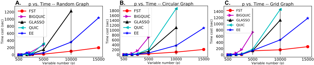
First, we apply FST and four baselines on synthetic data generated through varying p from {1000, 2500, 5000, 10000}, and fixing n = 2p and K = 20. All the methods are implemented with single thread in this experiment. Figure 2 implies that FST obtains significant computing time reduction compared to four provided baselines across all three data models. When p is large, FST is 2 ∼ 4 times faster than EE and is consistently 10 times around faster than GLasso, QUIC and BIGQUIC. The black dashed line in the figure indicates that GLasso, QUIC, and BIGQUIC are not able to obtain desired solutions in half an hour while FST needs much less time. The comparison of accuracy is also provided. Notice that GLasso and QUIC have the same solution and the solution of EE is the same as that in FST. Therefore, we only exhibit Frobenius-norm and max-norm of GLasso, FST and BIGQUIC. Table 2 shows that FST obtains the least Frobenius- and max-norm.
Moreover, we test the efficiency of FST in high-dimensional settings. In this experiment, we generate simulated datasets with p = 3000 and varies n from {1500, 2000, 3000}, each graph of which contains K = 20 random graphs. Notice that because the results reported in Table 2 indicate that BIGQUIC obtains worse solution than other methods, we omit BIGQUIC in this high-dimensional experiment and only compare the solution of FST with it of GLasso (or QUIC). In Table 3, it shows that FST obtains lower Frobenius-norm and max-norm under every conditions, denoting that FST outperforms other baselines in high-dimensional settings.
Furthermore, we evaluate our method on simulated datasets with millions of variables. Since other methods are infeasible for problems with a large number of variables, we only compare FST with EE and BIGQUIC using p = 106 , n = 104 and K = 40. We omit the computational cost for swapping blocks in and out of disks since the memory use in this experiment is relatively large. Table 4 shows that FST needs no more than 12 hours to finish running while BIGQUIC needs 24 hours using 32 threads.
| p | Time cost on fMRI datasets using 40 threads | ||
|---|---|---|---|
| FST | EE | GLasso | |
| 20480 | 207.2 secs | 382.5 secs | > 60 mins |
| 28672 | 794.4 secs | 1131.5 secs | > 60 mins |
| 36864 | 973.4 secs | 1696.6 secs | > 60 mins |
6.2 Experiment II: PrecisionMatrix Estimation on Real-World fMRI Data
We also evaluate FST and baselines for estimating precision matrices on a real-world fMRI dataset: SocialBrain [Tso et al., 2018]. This dataset is used to understand how the human brain processes social information. SocialBrain includes 120 samples, which are obtained through blood-oxygen-leveldependent imaging (BOLD) on 20480, 28672, 36864 voxels (i.e., variables). Like simulated experiments, all the tuning parameters are selected through 5-fold cross-validation. Table 5 shows that FST outperforms the other two baselines by using 40 cores (for this dataset). The estimated precision matrix is showed in Fig. 2 in the appendix. Results show that FST is able to obtain the graph's topological structure from fMRI datasets. Though the number of variables is less than one million, we show that our method is much faster than state-of-the-art ones.
7 Conclusion
This paper proposes FST, a scalable sparse Gaussian graphical model estimator with massive variables. By applying generalized thresholding to the sample covariance matrix, FST induces the true graphical topological structure and utilizes it to speed up estimation. Specifically, FST demonstrates its excellence by analyzing various topological graph structures, including cluster and social graphs. Theoretical analysis shows that FST obtains the same sharp convergence rate, O(√(logmax{p, n}/n), as most state-of-the-art methods while dramatically reducing the computational complexity to O(p2 ). Empirical experiments are used to validate that FST is faster than the baseline when achieving a lower error rate under both the Frobenius-norm and max-norm.
Acknowledgments
This work is supported by National Key R&D Program of China, 2018AAA0100500; National Natural Science Foundation of China under Grants, No. 61906040; the Natural Science Foundation of Jiangsu Province under grant BK20190335, BK20190345; National Natural Science Foundation of China under Grants , No. 61906037, 61972085; the Fundamental Research Funds for the Central Universities; Jiangsu Provincial Key Laboratory of Network and Information Security under Grants No.BM2003201, Key Laboratory of Computer Network and Information Integration of Ministry of Education of China under Grants No.93K-9.
@inproceedings{ijcai2020p410,
  title     = {Quadratic Sparse Gaussian Graphical Model Estimation Method for Massive Variables},
  author    = {Zhang, Jiaqi and Wang, Meng and Li, Qinchi and Wang, Sen and Chang, Xiaojun and Wang, Beilun},
  booktitle = {Proceedings of the Twenty-Ninth International Joint Conference on
               Artificial Intelligence, {IJCAI-20}},
  publisher = {International Joint Conferences on Artificial Intelligence Organization},
  editor    = {Christian Bessiere},
  pages     = {2964--2972},
  year      = {2020},
  month     = {7},
  note      = {Main track},
  doi       = {10.24963/ijcai.2020/410},
  url       = {https://doi.org/10.24963/ijcai.2020/410},
}
TY - CPAPER TI - Quadratic Sparse Gaussian Graphical Model Estimation Method for Massive Variables AU - Zhang, Jiaqi AU - Wang, Meng AU - Li, Qinchi AU - Wang, Sen AU - Chang, Xiaojun AU - Wang, Beilun T2 - Proceedings of the Twenty-Ninth International Joint Conference on Artificial Intelligence, IJCAI-20 PB - International Joint Conferences on Artificial Intelligence Organization PY - 2020 SP - 2964 EP - 2972 DO - 10.24963/ijcai.2020/410 UR - https://doi.org/10.24963/ijcai.2020/410 ER -Copied
Machine-readable versions of this paper, for tools and AI agents:





