
Modeling Trajectories with Neural Ordinary Differential Equations
Proceedings of the Thirtieth International Joint Conference on Artificial Intelligence. Main Track. Pages 1498-1504.
https://doi.org/10.24963/ijcai.2021/207
Keywords
- Multidisciplinary Topics and Applications: Ubiquitous Computing Systems
- Data Mining: Mining Spatial, Temporal Data
Abstract
Recent advances in location-acquisition techniques have generated massive spatial trajectory data. Recurrent Neural Networks (RNNs) are modern tools for modeling such trajectory data. After revisiting RNN-based methods for trajectory modeling, we expose two common critical drawbacks in the existing uses. First, RNNs are discrete-time models that only update the hidden states upon the arrival of new observations, which makes them an awkward fit for learning real-world trajectories with continuous-time dynamics. Second, real-world trajectories are never perfectly accurate due to unexpected sensor noise. Most RNN-based approaches are deterministic and thereby vulnerable to such noise. To tackle these challenges, we devise a novel method entitled TrajODE for more natural modeling of trajectories. It combines the continuous-time characteristic of Neural Ordinary Differential Equations (ODE) with the robustness of stochastic latent spaces. Extensive experiments on the task of trajectory classification demonstrate the superiority of our framework against the RNN counterparts.
- [Che et al., 2018] Zhengping Che, Sanjay Purushotham, Kyunghyun Cho, David Sontag, and Yan Liu. Recurrent neural networks for multivariate time series with missing values. Scientific reports, 8(1):1-12, 2018.
- [Chen et al., 2018] Ricky TQ Chen, Yulia Rubanova, Jesse Bettencourt, and David K Duvenaud. Neural ordinary dif- ferential equations. In Advances in neural information pro- cessing systems, pages 6571-6583, 2018.
- [De Brouwer et al., 2019] Edward De Brouwer, Jaak Simm, Adam Arany, and Yves Moreau. Gru-ode-bayes: Con- tinuous modeling of sporadically-observed time series. Advances in Neural Information Processing Systems, 32:7379-7390, 2019.
- [He et al., 2016] Kaiming He, Xiangyu Zhang, Shaoqing Ren, and Jian Sun. Deep residual learning for image recog- nition. In Proceedings of the IEEE conference on computer vision and pattern recognition, pages 770-778, 2016.
- [Huang et al., 2019] Xiaocheng Huang, Yifang Yin, Simon Lim, Guanfeng Wang, Bo Hu, Jagannadan Varadarajan, Shaolin Zheng, Ajay Bulusu, and Roger Zimmermann. Grab-posisi: An extensive real-life gps trajectory dataset in southeast asia. In Proceedings of the 3rd ACM SIGSPA- TIAL International Workshop on Prediction of Human Mo- bility, pages 1-10, 2019.
- [Kingma and Welling, 2013] Diederik P Kingma and Max Welling. Auto-encoding variational bayes. arXiv preprint arXiv:1312.6114, 2013.
- [Lechner and Hasani, 2020] Mathias Lechner and Ramin Hasani. Learning long-term dependencies in irregularly- sampled time series. Advances in neural information pro- cessing systems, 2020.
- [Liang et al., 2017] Yuxuan Liang, Zhongyuan Jiang, and Yu Zheng. Inferring traffic cascading patterns. In Proceed- ings of the 25th acm sigspatial international conference on advances in geographic information systems, pages 1-10, 2017.
- [Liu and Lee, 2017] Hongbin Liu and Ickjai Lee. End-to-end trajectory transportation mode classification using bi-lstm recurrent neural network. In 2017 12th International Con- ference on Intelligent Systems and Knowledge Engineer- ing (ISKE), pages 1-5. IEEE, 2017.
- [Liu et al., 2019] Hongbin Liu, Hao Wu, Weiwei Sun, and Ickjai Lee. Spatio-temporal gru for trajectory classifica- tion. In 2019 IEEE International Conference on Data Min- ing (ICDM), pages 1228-1233. IEEE, 2019.
- [Qin et al., 2019] Yanjun Qin, Haiyong Luo, Fang Zhao, Chenxing Wang, Jiaqi Wang, and Yuexia Zhang. Toward transportation mode recognition using deep convolutional and long short-term memory recurrent neural networks. IEEE Access, 7:142353-142367, 2019.
- [Rezende and Mohamed, 2015] Danilo Rezende and Shakir Mohamed. Variational inference with normalizing flows. In International Conference on Machine Learning, pages 1530-1538, 2015.
- [Ruan et al., 2020] Sijie Ruan, Cheng Long, Jie Bao, Chun- yang Li, Zisheng Yu, Ruiyuan Li, Yuxuan Liang, Tianfu He, and Yu Zheng. Learning to generate maps from trajec- tories. In Proceedings of the AAAI Conference on Artificial Intelligence, volume 34, pages 890-897, 2020.
- [Rubanova et al., 2019] Yulia Rubanova, Ricky TQ Chen, and David K Duvenaud. Latent ordinary differential equa- tions for irregularly-sampled time series. Advances in Neu- ral Information Processing Systems, 32:5320-5330, 2019.
- [Wu et al., 2017] Hao Wu, Ziyang Chen, Weiwei Sun, Bai- hua Zheng, and Wei Wang. Modeling trajectories with recurrent neural networks. In Proceedings of the Twenty- Sixth International Joint Conference on Artificial Intelli- gence, IJCAI-17, pages 3083-3090, 2017. IJCAI
- [Xu et al., 2017] Weidi Xu, Haoze Sun, Chao Deng, and Ying Tan. Variational autoencoder for semi-supervised text classification. In Proceedings of the AAAI Conference on Artificial Intelligence, volume 31, 2017.
- [Xu et al., 2018] Haowen Xu, Wenxiao Chen, Nengwen Zhao, Zeyan Li, Jiahao Bu, Zhihan Li, Ying Liu, Youjian Zhao, Dan Pei, Yang Feng, et al. Unsupervised anomaly detection via variational auto-encoder for seasonal kpis in web applications. In Proceedings of the 2018 World Wide Web Conference, pages 187-196, 2018.
- [Zheng et al., 2008a] Yu Zheng, Quannan Li, Yukun Chen, Xing Xie, and Wei-Ying Ma. Understanding mobility based on gps data. In Proceedings of the 10th interna- tional conference on Ubiquitous computing, pages 312- 321, 2008.
- [Zheng et al., 2008b] Yu Zheng, Like Liu, Longhao Wang, and Xing Xie. Learning transportation mode from raw gps data for geographic applications on the web. In Proceed- ings of the 17th international conference on World Wide Web, pages 247-256, 2008.
- [Zheng et al., 2010] Yu Zheng, Xing Xie, Wei-Ying Ma, et al. Geolife: A collaborative social networking service among user, location and trajectory. IEEE Data Eng. Bull., 33(2):32-39, 2010.
- [Zheng, 2015] Yu Zheng. Trajectory data mining: an overview. ACM Transactions on Intelligent Systems and Technology (TIST), 6(3):1-41, 2015.
- [Zhou et al., 2020] Fan Zhou, Liang Li, Kunpeng Zhang, Goce Trajcevski, Fuming Yao, Ying Huang, Ting Zhong, Jiahao Wang, and Qiao Liu. Forecasting the evolution of hydropower generation. In Proceedings of the 26th ACM SIGKDD International Conference on Knowledge Discov- ery & Data Mining, pages 2861-2870, 2020.
- [Zhu et al., 2017] Yu Zhu, Hao Li, Yikang Liao, Beidou Wang, Ziyu Guan, Haifeng Liu, and Deng Cai. What to do next: modeling user behaviors by time-lstm. In Pro- ceedings of the 26th International Joint Conference on Ar- tificial Intelligence, pages 3602-3608, 2017. IJCAI
References were extracted automatically from the PDF and may contain errors.
Full text extracted automatically from the PDF; figures, tables and equations may differ. The PDF is the version of record.
1 Introduction
A spatial trajectory is a sequence derived from a moving object in geographical spaces, formulated by a series of chronologically ordered points, i.e., T = p1 → p2 → · · · → pn. Each entry pi = (ai, bi, ti) contains a set of geospatial coordinates (i.e., longitude ai and latitude bi) and a timestamp ti ∈ R+. Modeling such trajectories allows us to analytically understand the moving objects and locations, facilitating a broad range of applications in smart transportation [Ruan et al., 2020] and trip recommendation [Zhu et al., 2017].
Recurrent Neural Networks (RNNs) are the modern tools for modeling spatial trajectories [Wu et al., 2017]. They are powerful in learning sequences with variable lengths and significantly reduce human effort in trajectory feature engineering, compared to traditional models such as SVMs and Random Forests [Zheng et al., 2008b]. Standard RNNs assume regular time intervals, while most trajectories are irregularlysampled due to many reasons like communication loads, battery issues, and weather conditions [Zheng, 2015]. To tackle a1 a2 b1 b2 b3 b4 b5 p5 p6 p4 p7 p8 p9 p10 this irregularity, a simple trick is to concatenate the time interval information to the input of RNNs [Liu and Lee, 2017; Qin et al., 2019]. As an alternative, GRU-D [Che et al., 2018] used an exponential decay mechanism on the hidden state until the next observation is made. Moreover, [Zhu et al., 2017; Che et al., 2018; Liu et al., 2019] enhanced RNNs with temporal gating mechanisms, where the time interval information is used to control the confidence of the input state.
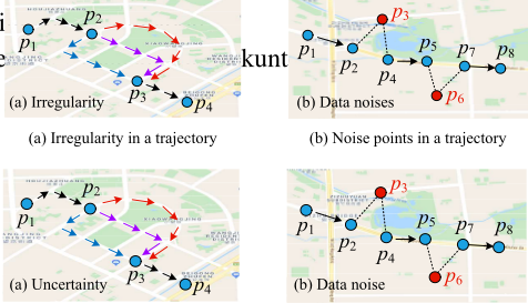
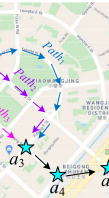
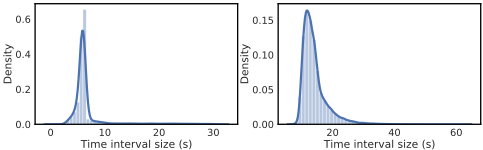
b6 b7 (b) Noise points in a trajectory Though RNNs with the aforementioned heuristics can address the irregularity to some extent, they are still insufficient for modeling real-world trajectories. That is because the time interval between irregular samples in real data can be tens of seconds or even several minutes (e.g., see Figure 6 for the interval distributions in two datasets). A larger interval induces larger uncertainty between observations, especially for highspeed moving objects. For example, as shown in Figure 1(a), the GPS coordinates of a car are recorded every few minutes, leading to multiple possible paths between two consecutive points (e.g., between p2 and p3). Since the existing RNN approaches can only update their states upon the occurrence of a new point, they cannot adequately model such uncertainty, resulting in degenerated performances. To better match reality, we need a method that can inherently consider the underlying continuous-time dynamics of the trajectories.
Moreover, trajectory data are never perfectly accurate due to atmospheric conditions and signal blockage [Zheng, 2015]. Figure 1(b) shows a trajectory with noise. Sometimes, these errors significantly impact model accuracy. Most of the RNN models for trajectory modeling are deterministic and infeasible to defeat such noise. An intuitive idea is to perform noise filtering [Zheng, 2015] before training our models. However, it requires extra human efforts to carefully specify the distance threshold and may significantly reduce the number of points in trajectories. Therefore, how to enhance the model robustness against data noise remains a challenge.
(c) Neural ODE
(d) TrajODE
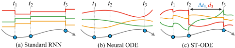
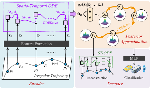
To address these issues, we present a novel model based on Neural Ordinary Differential Equations (ODE) for modeling trajectory data, entitled TrajODE. Targeting the first challenge, we devise a Spatio-Temporal ODE (ST-ODE) to model the continuous-time dynamics of a trajectory. As depicted in Figure 2(c), ST-ODE possesses continuous hidden states which obey an ODE between successive observations. Once a new point occurs, the state will be updated by a gating mechanism, which jointly considers the new input and the spatiotemporal interval since the last observation. To overcome the second challenge, we integrate ST-ODE with latent variables to enhance its robustness, where the whole model is trained with noise injected in its stochastic hidden layers, with a regularizer encouraging this noise injection. Furthermore, Continuous Normalizing Flows (CNF) [Chen et al., 2018] are incorporated to achieve a more unbiased posterior approximation. Compared to discrete layers in normalizing flows [Rezende and Mohamed, 2015], CNF uses instantaneous transformations to avoid expensive determinant computation by solving ODEs. In summary, our contributions are three-fold:
- To the best of our knowledge, we are the first to present an ODE-based approach (called ST-ODE) for modeling spatial trajectories, capturing the continuous-time dynamics in a principle way compared to RNN counterparts.
- Leveraging recent advances in deep variational models, we devise a novel framework entitled TrajODE for robust trajectory modeling by enhancing the proposed ST-ODE with latent variables, strengthening the robustness of our model against data noise by variational inference.
- We evaluate our approach on the trajectory classification task using two real-world mobility datasets. Compared to the state-of-the-art RNN approach, the results demonstrate that our model can improve the accuracy by 14% ∼ 21%.
2 RelatedWork
2.1 TrajectoryModeling
There has been a long line of studies in modeling trajectory data. [Zheng et al., 2008b] first applied several traditional algorithms (e.g., decision tree) to identify the transportation modes of a user's trajectory. They further identified a set of sophisticated features such as stop rate and velocity change to increase the classification accuracy [Zheng et al., 2008a]. Recently, RNNs have shown promising results in modeling trajectory data. In a pioneering study [Wu et al., 2017], the authors presented the first attempt to model trajectories by RNNs. Following this work, [Liu and Lee, 2017] employed bidirectional RNNs to recognize the transportation modes of GPS trajectories. To address the irregularity of trajectories, [Zhu et al., 2017; Che et al., 2018] extended RNNs to consider the time intervals between two consecutive points. [Liu et al., 2019] utilized 1D-CNN to model short-term spatial correlations between consecutive points, along with a time gating mechanism for learning spatio-temporal correlations. However, none of them can accurately model the continuoustime dynamics of a trajectory.
2.2 Neural Ordinary Differential Equations
Neural ODEs are a new family of deep learning models [Chen et al., 2018], which can be interpreted as a continuous equivalent of ResNet [He et al., 2016]. Recall that a residual layer updates the hidden state at time i by using a transformation f over the previous state, denoted as hi = hi-1 + f(hi-1). In contrast to this discrete update, Neural ODEs parameterize the derivative of the hidden state using a neural network fψ:
where ψ is the parameter set of f . In this way, the hidden state at any time τ can be evaluated via a blackbox ODE solver: h(τ ) = h(0) + ∫ τ 0 fψ(h(t), t)dt. We can simpify it as
where ODESolve is a numerical ODE solver, such as the Euler Method. Taking advantage of such models, ODE-RNNs [Rubanova et al., 2019], GRU-ODE-Bayes [De Brouwer et al., 2019] and ODE-LSTMs [Lechner and Hasani, 2020] enhanced RNNs to model irregularly-sampled time series. Inspired by these insightful studies, we present the first attempt to model spatial trajectories with Neural ODEs.
2.3 Deep Latent Variable Models
Deep latent variable models combine the approximation abilities of neural networks and the statistical foundations of generative models. Typically, Variational Autoencoders (VAEs) [Kingma and Welling, 2013] model the data distribution p(x) with the help of an unobserved latent variable z as a directed graphical model, i.e. p(x) = ∫ p(x|z)p(z)dz. As the integral is usually intractable, VAE implicitly optimizes the log-likelihood of the data by maximizing the evidence lower bound. A series of studies combined RNNs with VAEs for robust sequence modeling [Xu et al., 2017; Xu et al., 2018; Zhou et al., 2020]. Besides, [Rezende and Mohamed, 2015] developed Normalizing Flows (NF) for learning highly nonGaussian posterior densities by stacking a series of invertible transformations as zK = gK ◦ gK-1 ◦ · · · ◦ g1(z0), where each g is a bijective function. [Chen et al., 2018] further devised a continuous version of NF to reduce the computation cost by solving ODEs. Motivated by these previous studies, we equip our ST-ODE with latent variables to improve its robustness under the attack of GPS noise.
3 Methodology
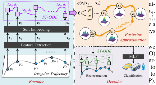
Given a trajectory T = p1 → p2 → · · · → pn, our task is to identify the mode of the whole trajectory. Figure 3 presents the framework of TrajODE for solving this problem, which consists of three major components:
- Encoder: We first perform feature extraction to obtain the features of each point (denoted as xi), and subsequently devise ST-ODE to learn high-level representations by modeling the continuous-time dynamics of the trajectory. Lastly, a fully-connected layer is used to transform the hidden state hi at each point to an output state oi, where i = 1, 2 . . . n.
3.1 Feature Extraction
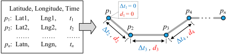
One of the main advantages of RNNs is that they can mitigate heavy feature engineering [Liu et al., 2019]. They directly feed the geospatial coordinates (ai, bi) and timestamp ti into each RNN unit to learn high-level representations. In this study, we propose to extract several simple yet useful features to boost the model performance. We attach the attributes of each segment to its termination point. As shown in Figure 4, we first compute the time interval ∆ti = ti - ti-1 and the geospatial distance di between two consecutive points pi-1 and pi. As the speed and acceleration of a moving object can determine the transportation modes, we approximate the velocity of each segment by vi = di/∆ti and compute the acceleration using ri = |vi -vi-1|/∆ti. Finally, we concatenate them with the geospatial coordinates as the feature of the i-th point xi = [ai, bi, vi, ri] ∈ R4 . The spatio-temporal interval (∆ti, di) will also be used in the following section.
3.2 Spatio-Temporal ODE
When applying Neural ODEs to modeling GPS trajectories, a major issue is that the solution to an uncontrolled ODE is only determined by its initial condition, and we cannot adjust the hidden states based on subsequent observations. To this end, ODE-RNNs provide a new paradigm for learning irregularlysampled data. The main idea is to employ a black-box ODE solver to evaluate the hidden state between successive records and a standard RNN cell to update its state at observations:
where h′i ∈ Rm is the solution at ti to an ODE started from ti-1; hi ∈ Rm is the updated hidden state.
However, we notice that the time lapse between successive GPS points can vary from seconds to minutes in trajectories, e.g., in GeoLife dataset [Zheng et al., 2010]. As the time interval increases, it will be more difficult for the ODE solver to evaluate the continuous hidden dynamics (Eq. 3), which implies that we should believe more in the current observation. Similarly, the spatial interval (i.e., distance) between consecutive points also affects the confidence of the ODE states. According to Eq. 4, ODE-RNN leverages a simple shared RNN cell to update the hidden state at any time step, making it fail to capture the impact of various spatio-temporal intervals.
Based on the above findings, we present an ST-ODE model to learn the continuous-time dynamics while considering such spatio-temporal interval information by a gating mechanism. The procedures are illustrated in Algorithm 1. First, we follow [Lechner and Hasani, 2020] to employ an LSTM before performing the ODE solver to avoid the vanishing or exploding of gradients (line 3), where the soft embedding achieved by LSTM at ti is denoted as ei ∈ Rm. Then, we obtain the ODE state at each time step by solving ODEs in line 4. Given the ODE state h′i and the current embedding ei, we update hi using the proposed gating mechanism (line 5):
where the spatio-temporal (ST) gate ui ∈ Rm is a function w.r.t. the ST interval (∆ti and di), which helps the model to determine how much of the state solved by ODE needs to be passed along to the future. Instead of using a fixed priori like e-(∆ti+λdi) [Liang et al., 2017], we parameterize it to be
where Wu ∈ R2×m and bu ∈ Rm are learnable parameters. Such computation ensures each decay rate monotonically decreases in a reasonable range between 0 and 1. Finally, we compute the output states {o1 . . . on} via a fully-connected layer (line 6) for downstream applications, where oi ∈ Rm.
Algorithm 1: The ST-ODE model
Input: {(xi, ti, ∆ti, di)}i=1...n
Output: The output state {oi}i=1...n
1 h0 = c0 = 0 ▷ Initialize hidden state and memory cell.
2 for i = 1 . . . n do
3 (ei, ci) = LSTMCell(xi, (hi-1, ci-1))
4 h′i = ODESolve (fψ, hi-1, (ti-1, ti))
5 hi = ST-Gate(ei, h′i,∆ti, di)
6 oi =Wohi +bo whereWo ∈ Rm×m, bo ∈ Rm
7 end
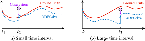
To help better understand how ST-ODE works, Figure 5 depicts an example of the ground truth (red line) and the ODE curves (blue line) of hidden states in ST-ODE. When the time interval is small (between t1 and t2), the error of hidden state (the margin between the two lines) is acceptable, thereby allowing more parts of the ODE state passing through the gate. On the contrary, when the time interval is very large (from t1 to t3), we should believe more in the new observation rather than the ODE state at t3. The sample principle holds true if it extends to cases with different spatial intervals.
3.3 Posterior Approximation
Different from the deterministic RNNs for classification, our TrajODE approximates the complex posterior distribution of the latent variables z to enhance its robustness. Let pθ(z0|X) be the true posterior distribution, where X = {x1 . . . xn} is the point features. We follow VAEs to approximate pθ(z0|X) with qφ(z0|X) using a neural network model, where φ is the parameter set of q. We first derive the mean µ ∈ Rm and variance σ ∈ Rm of latent variable z0 from the output of ST-ODE (on) using linear transformations. Going along with the reparameterization trick [Kingma and Welling, 2013], we sample the latent variable z0 from qφ(z0|X) by z0 = µ+σϵ, where ϵ ∼ N(0, 1) and zo ∈ Rm.
However, the estimated posterior qφ(z0|X) in vanilla VAE is restricted to obey a normal distribution, which makes it hard to reflect the real characteristics of trajectory data. A natural idea is using normalizing flows (NF) [Rezende and Mohamed, 2015], where a series of invertible mappings g1 . . . gK are performed to convert the initial known distribution to a more complicated one. Given the initial latent variable z0, the probability of the output variable zK = gK ◦ gK-1 ◦ · · · ◦ g1(z0) is given by the change of variable theorem:
where z0 can be computed from zK using the inverse flow z0 = g-1 1 ◦ g-1 2 ◦ · · · ◦ g-1 K (zK). However, it requires cubic cost in computing the determinant of the Jacobian ∂gk/∂zk.
Inspired by recent advances in Neural ODEs, we introduce a continuous normalizing flow (CNF) [Chen et al., 2018] to enable our model approximate more accurate posterior distribution (thereby more robust against noise), while avoiding the cubic cost in the determinant computation. In contrast to discrete transformations in NF, we define each mapping as a continuous-time dynamic: dz(k) dk = gω(z(k), k), i.e., a differential equation gω that can be parameterized by a neural network. Based on the theorem of instantaneous change of variables [Chen et al., 2018], the change in the log probability also follows a differential equation:
where tr represents the trace operation, reducing the cubic cost to a linear cost with regard to the number of hidden units. By using Eq. 8, the latent variable after a time period with length K can be computed as zK = z0 + ∫ K 0 gω (zk, k) dk, while its log distribution can be written as:
In this way, we can learn a more accurate non-Gaussian posterior qφ(zK|X) compared to the original one, i.e., qφ(z0|X). As this procedure is continuous, we set K = 1 for simplicity.
3.4 Decoders &Optimization
After posterior approximation, we apply a 2-layer MLP with 64 hidden units as classifier to generate the prediction ˆy from the latent variable zK. Then, another ST-ODE is used as the decoder to reversely reconstruct the raw trajectory from the latent variable zK, which measures the reconstruction likelihood Eqφ log [pθ (X|zK)] based on the variational posterior distribution. Here, we do not treat the reconstruction task as an initial-value problem since directly using Neural ODEs for reconstruction performs badly in our experiments.
When performing back-propagation, computing the gradients of Neural ODEs is memory prohibitive as the states are infinitely many over time. We address this issue with the adjoint sensitivity method [Chen et al., 2018], which results in only O(1) memory cost. Let Ω be the learnable parameters, we train our model by jointly minimizing two loss functions:
where LCE denotes the cross-entropy loss between the prediction ˆy and ground truth y; the second term LELBO means the evidence lower bound, which is computed as;
where the first term is the reconstruction likelihood; the last three terms represent the KL Divergence of the prior distribution and the variational posterior distribution.
4 Experiments
4.1 Datasets
We conduct our experiments over two public datasets:
- GeoLife [Zheng et al., 2010]: GeoLife contains 17,621 trajectories collected by 182 users from a peroid of five years (from 2007 to 2012). Among them, 73 users have labeled part of their trajectories with transportation modes. Following [Liu et al., 2019], our target is to identify the travel modes (i.e, walking, bike, bus and car) of a trajectory.
- Grab-Posisi [Huang et al., 2019]: This dataset is sampled from Grab 1 drivers' trajectories in Singapore and Jakarta. The data in Jakarta provide two transportation modes (car or motorcycle). We choose the data ranging from 2019-0410 to 2019-04-13 for the binary classification task.
After preprocessing, we obtain 15,639 and 119,551 instances ranging from 5 to 30 minutes from the two datasets, respectively. Each of them possesses 20 to 100 GPS points. Figure 1 illustrates the distribution of time intervals in these datasets. The time interval in Grab-Posisi is generally larger than that in GeoLife, which aggravates the irregularity and thereby increases the difficulty of modeling. For both datasets, we partition the data into training, validation and test data by a ratio of 8:1:1. Z-score normalization is performed on inputs for fast training. See more details in our Data Appendix.
4.2 Experimental Settings
Baselines
We consider nine baselines that belong to three classes:
- Traditional models: We follow [Zheng et al., 2008b] to implement SVM and Random Forest (RF) for comparison. The classification is based on the extracted metadata, e.g., the mean/variance of velocity and acceleration.
- RNN approaches: We take the RNN models introduced in Section 2.1 as RNN baselines, including RNN, BiLSTM [Liu and Lee, 2017], TimeLSTM [Zhu et al., 2017], GRUD [Che et al., 2018], and STGRU [Liu et al., 2019].
- Neural ODEs: LatentODE [Rubanova et al., 2019] and ODE-LSTM [Lechner and Hasani, 2020] are variants of ODE-RNN for modeling irregularly-sampled time series, which can be easily adapted to our classification task.
For RNN and ODE-RNN based models, we sequentially feed each GPS point pi = (ai, bi, ti) into the corresponding RNN unit for learning representations. To be fair, we also employ a subnetwork to fuse the metadata at the top of these models to increase their classification accuracy.
1 Grab is a ride-sharing company based in Singapore.
Implementation Details & Hyperparameters
We implement TrajODE and the baselines with PyTorch 1.7. Our model is trained by an Adam optimizer with an initial learning rate of 0.01, reduced by 1/10 every 20 epochs. The batch size is 128 and 512 over the two datasets, respectively. For simplicity, we use the same hidden dimensionality at the encoder and decoder, and conduct a grid search for m from 16 to 512. The ODE solvers in both ST-ODE and CNF are the Euler Method, where the evaluation functions are 3-layer MLPs with m hidden units in each layer. The trade-off parameter (γ) in Eq. 10 is set as 5e - 4. As the observation times are different for each trajectory in a batch, we solve all ODEs in a batch by computing the solution of the combined ODE at the union of all timestamps in the batch.
Evaluation Metrics
We follow [Zheng et al., 2008b; Liu et al., 2019] to employ the classification accuracy (Acc) to evaluate model performance. For each dataset, we run each method 5 times and report the mean accuracy of each model. We also use the notation ∆ to indicate the relative improvement of accuracy compared with the state-of-the-art RNN method, i.e., STGRU.
4.3 Model Comparison
In this section, we compare our model with the baselines over the two datasets. We present the best performance of each method under different hyperparameter settings in Table 1. For example, we report the results of TrajODE with m = 64 as our default settings on both datasets.
It can be seen easily that our TrajODE clearly outperforms all the baselines over both datasets. Compared to the state-ofthe-art RNN method (STGRU), TrajODE improves the accuracy by 20.9% and 13.6% on the two datasets, respectively. The reasons are two-fold. First, TrajODE captures the uncertainty between observations via a continuous-time approach, resulting in more accurate and natural modeling of trajectories. Second, TrajODE takes advantage of the variational inference to be less vulnerable to the attack of data noise. From this table, we can also observe that: 1) Directly using Neural ODEs like ODE-LSTM cannot bring significant improvements against RNNs, since they are originally designed for irregularly-sampled time series which are not the case for GPS trajectories (containing both spatial and temporal intervals). 2) In contrast to GeoLife, the performances of RNN variants are not very distinctive in Grab-Posisi due to its larger time intervals (see Figure 6). 3) Stochastic approaches (i.e., TrajODE and LatentODE) achieve better performance than those deterministic models, which demonstrates the robustness provided by the stochastic latent space.
| Method | GeoLife | Grab-Posisi | ||
|---|---|---|---|---|
| Acc | ∆ | Acc | ∆ | |
| SVM RF | 0.526 0.592 | -22.0% -12.2% | 0.552 0.562 | -21.8% -20.4% |
| RNN BiLSTM GRU-D STGRU | 0.629 0.638 | -6.7% -5.3% | 0.704 0.690 | -12.5% -0.3% -2.3% |
| TimeLSTM | 0.614 | -8.9% | 0.618 | |
| -2.6% | ||||
| 0.625 | -7.3% | 0.688 | ||
| 0.674 | - | 0.706 | - | |
| LatentODE | 0.715 | +6.1% | 0.733 | +3.8% |
| ODE-LSTM | 0.645 | -4.3% | 0.698 | -1.1% |
| TrajODE | 0.815 | +20.9% | 0.802 | +13.6% |
4.4 Variant Comparison
To further investigate the effectiveness of each model component, we compare TrajODE with its variants as follows:
- TrajODE-RNN: This variant employs RNNs as the encoder and decoder rather than using ST-ODEs.
- TrajODE-ODE-RNN: We replace ST-ODEs with ODERNNs for encoding and decoding the trajectories.
- TrajODE-w/o PA: We remove the posterior approximation from TrajODE to validate its efficacy, i.e., we only use STODE as a deterministic method for trajectory classification.
- TrajODE-w/o CNF: To evaluate the CNF for learning nonGaussian posterior distribution, we directly turn it off.
Evaluation on Feature Extraction
We first check if the features that we feed into TrajODE are really useful. As shown in Table 2, we add locations (Fl), approximated velocity (Fv) and acceleration (Fr) step by step. Although these features look simple, we see a clear improvement in the model accuracy while not increasing the model complexity. In particular, we also follow [Liu and Lee, 2017] to concatenate the locations with the time interval information for comparison (denoted by Fl+t). The results show integrating with velocity and acceleration contributes more to the classification task than the time interval information.
| Features | Fl | Fl+v | Fl+r | Fl+v+r | Fl+t |
|---|---|---|---|---|---|
| GeoLife | 0.791 | 0.806 | 0.799 | 0.815 | 0.795 |
| Grab-Posisi | 0.776 | 0.796 | 0.788 | 0.802 | 0.782 |
Evaluation on ST-ODE
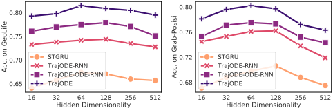
As the major building block of our model, ST-ODE enables us to model the continuous-time dynamics of trajectories. Here, we attempt STGRU and the variants of TrajODE with different hidden dimensionality (m) to verify the efficacy of STODE. Figure 7 shows the comparison results, from which we can have the following observations. First, TrajODE consistently outperforms both variants over all hidden state sizes by jointly capturing the continuous-time dynamics and the spatio-temporal intervals between observations. For example, the improvement of TrajODE over TrajODE-ODE-RNN can verify the efficacy of our ST gating mechanism. Second, the performance of TrajODE and its variants are not very sensitive to the hidden dimensionality in GeoLife. Third, TrajODE with m = 64 achieves the best performance in both datasets. As m exceeds 128, it will induce much more trainable parameters and lead to an overfitting problem. Thus, we choose m = 64 as the default setting of our model.
Evaluation on Posterior Approximation
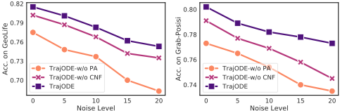
As this component is employed to enhance the model robustness against data noise, we thereby evaluate it under different noise levels. We use a normal distribution N(0, λ2 ) to generate an offset for each GPS point, where λ is the standard deviation (in meters) and can be interpreted as the noise level. As shown in Figure 8, the accuracy of each model decreases with the increase of λ over both datasets. TrajODE achieves much higher accuracy in all levels of noise compared to the deterministic model (TrajODE-w/o PA), which reveals the superiority of integrating with stochastic latent space. Moreover, TrajODE outperforms its variant w/o CNF by a considerable margin because CNF allows the latent variables zK obeying a more complex posterior distribution.
5 Conclusion and FutureWork
In this paper, we devise a continuous-time model called TrajODE with latent variables for modeling spatial trajectories. It possesses continuous states between observations, and also updates the hidden state by new observations while considering the spatio-temporal intervals. Meanwhile, the latent variable space enhances the model robustness against the data noise. Compared to the state-of-the-art RNNs, TrajODE improves the classification accuracy by approximately 14% to 21% on two real-world mobility datasets. However, we have noticed that the major efficiency bottleneck is the evaluation between two observations. In the future, we plan to reduce the number of function evaluations in the ODE solver while preserving the model accuracy, and explore TrajODE on other downstream applications, such as trajectory prediction.
Acknowledgments
This research is supported by Singapore Ministry of Education Academic Research Fund Tier 2 under MOE's official grant number MOE2018-T2-1-103. We thank all reviewers for their constructive suggestions in improving this paper.
@inproceedings{ijcai2021p207,
  title     = {Modeling Trajectories with Neural Ordinary Differential Equations},
  author    = {Liang, Yuxuan and Ouyang, Kun and Yan, Hanshu and Wang, Yiwei and Tong, Zekun and Zimmermann, Roger},
  booktitle = {Proceedings of the Thirtieth International Joint Conference on
               Artificial Intelligence, {IJCAI-21}},
  publisher = {International Joint Conferences on Artificial Intelligence Organization},
  editor    = {Zhi-Hua Zhou},
  pages     = {1498--1504},
  year      = {2021},
  month     = {8},
  note      = {Main Track},
  doi       = {10.24963/ijcai.2021/207},
  url       = {https://doi.org/10.24963/ijcai.2021/207},
}
TY - CPAPER TI - Modeling Trajectories with Neural Ordinary Differential Equations AU - Liang, Yuxuan AU - Ouyang, Kun AU - Yan, Hanshu AU - Wang, Yiwei AU - Tong, Zekun AU - Zimmermann, Roger T2 - Proceedings of the Thirtieth International Joint Conference on Artificial Intelligence, IJCAI-21 PB - International Joint Conferences on Artificial Intelligence Organization PY - 2021 SP - 1498 EP - 1504 DO - 10.24963/ijcai.2021/207 UR - https://doi.org/10.24963/ijcai.2021/207 ER -Copied
Machine-readable versions of this paper, for tools and AI agents:





