
What to Do Next: Modeling User Behaviors by Time-LSTM
Proceedings of the Twenty-Sixth International Joint Conference on Artificial Intelligence. Main track. Pages 3602-3608.
https://doi.org/10.24963/ijcai.2017/504
Keywords
- Machine Learning: Time-series/Data Streams
- Machine Learning: Deep Learning
- Machine Learning: Data Mining
Abstract
Recently, Recurrent Neural Network (RNN) solutions for recommender systems (RS) are becoming increasingly popular. The insight is that, there exist some intrinsic patterns in the sequence of users' actions, and RNN has been proved to perform excellently when modeling sequential data. In traditional tasks such as language modeling, RNN solutions usually only consider the sequential order of objects without the notion of interval. However, in RS, time intervals between users' actions are of significant importance in capturing the relations of users' actions and the traditional RNN architectures are not good at modeling them. In this paper, we propose a new LSTM variant, i.e. Time-LSTM, to model users' sequential actions. Time-LSTM equips LSTM with time gates to model time intervals. These time gates are specifically designed, so that compared to the traditional RNN solutions, Time-LSTM better captures both of users' short-term and long-term interests, so as to improve the recommendation performance. Experimental results on two real-world datasets show the superiority of the recommendation method using Time-LSTM over the traditional methods.
- [Aghabozorgi and Wah, 2009] Saeed R Aghabozorgi and Teh Ying Wah. Recommender systems: incremental clus- tering on web log data. In ICIS, pages 812-818. ACM, 2009.
- [AlMurtadha et al., 2010] Yahya AlMurtadha, M.N.B. Su- laiman, Norwati Mustapha, Nur Izura Udzir, and Zaiton Muda. Ars: Web page recommendation system for anony- mous users based on web usage mining. In Proc. ECS, volume 10, pages 115-120, 2010.
- [Cho et al., 2014] Kyunghyun Cho, Bart Van Merriënboer, Caglar Gulcehre, Dzmitry Bahdanau, Fethi Bougares, Holger Schwenk, and Yoshua Bengio. Learning phrase representations using rnn encoder-decoder for statistical machine translation. arXiv:1406.1078, 2014.
- [Duchi et al., 2011] John Duchi, Elad Hazan, and Yoram Singer. Adaptive subgradient methods for online learning and stochastic optimization. JMLR, 12(Jul):2121-2159, 2011.
- [Gers and Schmidhuber, 2000] Felix A Gers and Jürgen Schmidhuber. Recurrent nets that time and count. In IJCNN, volume 3, pages 189-194. IEEE, 2000.
- [Graves, 2013] Alex Graves. Generating sequences with re- current neural networks. arXiv:1308.0850, 2013.
- [Greff et al., 2016] Klaus Greff, Rupesh K Srivastava, Jan Koutník, Bas R Steunebrink, and Jürgen Schmidhuber. Lstm: A search space odyssey. IEEE TNNLS, 2016.
- [He et al., 2015] Kaiming He, Xiangyu Zhang, Shaoqing Ren, and Jian Sun. Delving deep into rectifiers: Surpass- ing human-level performance on imagenet classification. In ICCV, pages 1026-1034, 2015.
- [Hidasi et al., 2016a] Balázs Hidasi, Alexandros Karat- zoglou, Linas Baltrunas, and Domonkos Tikk. Session- based recommendations with recurrent neural networks. In ICLR, 2016.
- [Hidasi et al., 2016b] Balázs Hidasi, Massimo Quadrana, Alexandros Karatzoglou, and Domonkos Tikk. Paral- lel recurrent neural network architectures for feature-rich session-based recommendations. In RecSys, pages 241- 248. ACM, 2016.
- [Hochreiter and Schmidhuber, 1997] Sepp Hochreiter and Jürgen Schmidhuber. Long short-term memory. Neural computation, 9(8):1735-1780, 1997.
- [Huang et al., 2004] Xiangji Huang, Fuchun Peng, Aijun An, and Dale Schuurmans. Dynamic web log session iden- tification with statistical language models. Journal of the American Society for Information Science and Technology, 55(14):1290-1303, 2004.
- [Jannach et al., 2015] Dietmar Jannach, Lukas Lerche, and Michael Jugovac. Adaptation and evaluation of recom- mendations for short-term shopping goals. In RecSys, pages 211-218. ACM, 2015.
- [Janssen and Limnios, 2013] Jacques Janssen and Nikolaos Limnios. Semi-Markov models and applications. Springer Science & Business Media, 2013.
- [Koren et al., 2009] Yehuda Koren, Robert Bell, and Chris Volinsky. Matrix factorization techniques for recom- mender systems. Computer, 42(8), 2009.
- [Liu et al., 2010] Jiahui Liu, Peter Dolan, and Elin Rønby Pedersen. Personalized news recommendation based on click behavior. In IUI, pages 31-40. ACM, 2010.
- [Mikolov et al., 2010] Tomas Mikolov, Martin Karafiát, Lukas Burget, Jan Cernockỳ, and Sanjeev Khudanpur. Re- current neural network based language model. In Inter- speech, volume 2, page 3, 2010.
- [Neil et al., 2016] Daniel Neil, Michael Pfeiffer, and Shih- Chii Liu. Phased lstm: Accelerating recurrent network training for long or event-based sequences. In NIPS, pages 3882-3890, 2016.
- [Rakhlin et al., 2012] Alexander Rakhlin, Ohad Shamir, and Karthik Sridharan. Making gradient descent optimal for strongly convex stochastic optimization. In ICML, pages 449-456, 2012.
- [Rendle et al., 2009] Steffen Rendle, Christoph Freuden- thaler, Zeno Gantner, and Lars Schmidt-Thieme. Bpr: Bayesian personalized ranking from implicit feedback. In UAI, pages 452-461. AUAI Press, 2009.
- [Tan et al., 2016] Yong Kiam Tan, Xinxing Xu, and Yong Liu. Improved recurrent neural networks for session-based recommendations. In RecSys, pages 17-22. ACM, 2016.
- [Wang et al., 2016a] Beidou Wang, Martin Ester, Jiajun Bu, Yu Zhu, Ziyu Guan, and Deng Cai. Which to view: Per- sonalized prioritization for broadcast emails. In WWW, pages 1181-1190, 2016.
- [Wang et al., 2016b] Beidou Wang, Martin Ester, Yikang Liao, Jiajun Bu, Yu Zhu, Ziyu Guan, and Deng Cai. The million domain challenge: Broadcast email prioritization by cross-domain recommendation. In KDD, pages 1895- 1904. ACM, 2016.
- [Yu et al., 2016] Feng Yu, Qiang Liu, Shu Wu, Liang Wang, and Tieniu Tan. A dynamic recurrent model for next basket recommendation. In SIGIR, pages 729-732. ACM, 2016.
- [Zhao et al., 2015] Zhou Zhao, Ruihua Song, Xing Xie, Xi- aofei He, and Yueting Zhuang. Mobile query recommen- dation via tensor function learning. In IJCAI, volume 15, pages 4084-4090, 2015. IJCAI
- [Zhao et al., 2016] Zhou Zhao, Hanqing Lu, Deng Cai, Xi- aofei He, and Yueting Zhuang. User preference learning for online social recommendation. TKDE, 28(9):2522- 2534, 2016.
- [Zhu et al., 2016] Yu Zhu, Ziyu Guan, Shulong Tan, Haifeng Liu, Deng Cai, and Xiaofei He. Heterogeneous hyper- graph embedding for document recommendation. Neuro- computing, 216:150-162, 2016.
References were extracted automatically from the PDF and may contain errors.
Full text extracted automatically from the PDF; figures, tables and equations may differ. The PDF is the version of record.
1 Introduction
Recurrent Neural Network (RNN) solutions have become state-of-the-art methods on modeling sequential data. They are applied to a variety of domains, ranging from language modeling to machine translation to image captioning. With remarkable success achieved when RNN is applied to aforementioned domains, there is an increasing number of works trying to find RNN solutions in the area of recommender systems (RS). [Hidasi et al., 2016a; Tan et al., 2016; Hidasi et al., 2016b] focus on RNN solutions in one certain type of recommendation task, i.e. session-based recommendations, where no user id exists and recommendations are based on previous consumed items within the same session. [Yu et al., 2016] points out that RNN is able to capture users' general interest and sequential actions in RS and designs a RNN method for the next-basket recommendations. The insight that RNN works well in the above recommendation tasks is that, there exist some intrinsic patterns in the sequence of users' actions, e.g. once a man buys a badminton racket, he tends to buy some badmintons later, and RNN has been proved to perform excellently when modeling this type of patterns.
∗ corresponding author
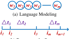
Figure 1: wm in (a) represents the m-th word. In (b), im represents the m-th consumed item and △tm is the time interval between the time when im and im+1 are consumed.
However, none of the above RNN solutions in RS considers the time interval between users' neighbour actions, while these time intervals are important to capture the relations of users' actions, e.g. two actions within a short time tend to be related and actions with a large time interval may aim at different goals. Therefore, it is important to exploit the time information when modeling users' behaviors, so as to improve the recommendation performance. We use Figure 1 to show what the time interval is and how it makes RS different from the traditional domains such as language modeling. Specifically, there is no notion of interval between neighbour words (e.g. no interval between w1 and w2) in language modeling, while there are time intervals between neighbor actions (e.g. △t1 between i1 and i2) in RS. Traditional RNN architectures are good at modeling the order information of sequential data as in Figure 1 (a), but they cannot well model time intervals in Figure 1 (b). Therefore, new models need to be proposed to address this problem.
A recently proposed model, i.e. Phased LSTM [Neil et al., 2016], tries to model the time information by adding one time gate to LSTM [Hochreiter and Schmidhuber, 1997], where LSTM is an important ingredient of RNN architectures. In this model, the timestamp is the input of the time gate which controls the update of the cell state, the hidden state and thus the final output. Meanwhile, only samples lying in the model's active state are utilized, resulting in sparse updates during training. Thus, Phased LSTM can obtain a rather fast learning convergence in the training phase. However, there exist several challenges preventing Phased LSTM from becoming the best fit for recommendation tasks.
First of all, Phased LSTMmodels the timestamp, which is the characteristic of one single action, rather than the time interval between two actions. Hence, Phased LSTM may fail to properly model actions' relations. Secondly, users' action data is usually very sparse in most RS and Phased LSTM would ignore users' actions in its inactive state, which cannot make full use of behaviors' information for recommendations. Thirdly, previous studies [Jannach et al., 2015] have pointed out that both of users' short-term and long-term interests are of great importance for recommendations, but traditional RNN architectures (including Phased LSTM) are not designed to distinguish and exploit these two types of interests simultaneously. Here, the short-term interest means that, the recommended items should depend on recently consumed items. For example, if a user just buys a Nikon camera, he is very likely to pick-up a memory card, lenses and protection cases in the near future. The long-term interest means that the recommended items should also be influenced by users' past actions, which reflect users' general interest.
To cope with the above challenges, we propose TimeLSTM, with three versions, to model users' sequential actions in RS. Actions' time intervals are modeled by time gates in Time-LSTM to capture actions' relations. The first version has only one time gate, which exploits time intervals to simultaneously capture the short-term and long-term interests. There are two time gates in our second version. One is designed to exploit time intervals to capture the short-term interest for current item recommendations and the other is to save time intervals to model the long-term interest for later recommendations. In the third version, we use coupled input and forget gates [Greff et al., 2016] to reduce the number of parameters, making our model more concise. TimeLSTM with these time gates well captures users' short-term and long-term interests at the same time, so as to improve the recommendation performance. In addition, Time-LSTM has no inactive state to ignore actions, so that compared to Phased LSTM, it can make better use of behaviors' information. Our experimental results demonstrate the effectiveness of TimeLSTM. The contributions of this paper are as follows:
- Our proposed model, Time-LSTM, equips LSTM with carefully designed time gates, so that it is not only good at modeling the order information in sequential data, but can also well capture the interval information between objects. This is a general idea (not limited to RS) and other variants of Time-LSTM could be developed to model the event-based sequential data [Neil et al., 2016] in other tasks. Note that different from Phased LSTM, which considers the timestamp and may implicitly capture the interval information, we explicitly model time intervals. In addition, compared to Phased LSTM, TimeLSTM exploits the information of more samples.
- We propose three versions of Time-LSTM. Compared to existing RNN solutions, these Time-LSTM versions can better capture users' short-term and long-term interests at the same time, so as to improve the recommendation
performance.
- Our proposed models are evaluated on two real-world datasets, and the experimental results show the superiority of the recommendation method using Time-LSTM over traditional methods.
2 RalatedWork
2.1 LSTMand Its Variants
LSTM: The commonly-used update equations [Graves, 2013] of LSTM are as follows:
cm = fm ⊙ cm-1
where im, fm, om represent the input, forget and output gates of the m-th object respectively. cm is the cell activation vector. xm and hm represent the input feature vector and the hidden output vector respectively. Typically, σi, σf , σo are sigmoidal nonlinearities and σc, σh are tanh nonlinearities. Weight parameters Whi, Whf , Who, Wxi, Wxf and Wxo connect different inputs and gates with memory cells and outputs. bi, bf and bo are corresponding biases. The update equation of cm has two parts, one is a fraction of the previous cell state cm-1 that is controlled by fm, and the other is a new input state created from the element-wise (Hadamard) product, denoted by ⊙, of im and the output of the nonlinearity σc. The operation of input, forget and output gates can be further influenced by optional peephole [Gers and Schmidhuber, 2000] connection weights wci, wcf , wco.
Coupled input and forget gates: One variant of LSTM is to use coupled input and forget gates [Greff et al., 2016] instead of separately deciding what to forget and what new information to add. It drops Eq. (2) and modifies Eq. (3) to:
Phased LSTM: Phased LSTM [Neil et al., 2016] is a state-ofthe-art RNN architecture for modeling event-based sequential data. It extends LSTM by adding the time gate km. km is controlled by three parameters: τ, ron and s, where τ represents the total period of the model, s represents the phase shift and ron is the ratio of the open period to the total period. τ, ron and s are learned by training. km is formally defined as:
where tm is the timestamp and φm is an auxiliary variable. The gate km has three phases: km rises from 0 to 1 in the first phase and drops from 1 to 0 in the second phase (active state).
During the third phase, the model is in the inactive state. The leak rate α (close to 0 in training and equal to 0 in testing) is to propagate gradient information [He et al., 2015]. Updates to cm and hm are permitted only in the active state. It rewrites Eq. (3) and Eq. (5) in LSTM to:
Due to the setting of inactive state, Phased LSTM cannot make full use of users' actions when applied to RS.
2.2 RNN Solutions in RS
[Hidasi et al., 2016a; Tan et al., 2016; Hidasi et al., 2016b] focus on RNN solutions in session-based recommendations. [Hidasi et al., 2016a] trains RNN with a ranking loss on onehot representations of item-IDs in old sessions. The RNN is then used to provide recommendations on new user sessions. [Tan et al., 2016] is an extension to [Hidasi et al., 2016a], where it proposes two techniques, i.e. data augmentation and a method to account for shifts in the input data distribution, to improve the model performance. [Hidasi et al., 2016b] considers a slightly different setting, where items' rich features exist. It introduces parallel RNN architectures to model clicks and items' features. [Yu et al., 2016] designs a RNNmethod for the next-basket recommendations.
In this paper, we explore RNN solutions with a more common setting in the RS community, where we know the user id, but no session information is known. [Yu et al., 2016] directly applies RNN to RS, without considering time intervals, while we add time gates to LSTM, which can exploit time intervals to improve the recommendation performance.
2.3 The Short-term and Long-term Interests
Most existing algorithms in RS, e.g. BPR (Bayesian Personalized Ranking) [Rendle et al., 2009], matrix factorization [Koren et al., 2009], tensor models [Zhao et al., 2015], focus on modeling users' long-term interest, while the short-term interest seems to play a minor role in RS research. [Liu et al., 2010] adapts a collaborative filtering approach to the user's current interest mined by content-based methods. Some approaches, e.g. [Aghabozorgi and Wah, 2009], [AlMurtadha et al., 2010], apply collaborative filtering and association rules to match users' recent actions. [Jannach et al., 2015] proposes that both of users' short-term and long-term interests are important in online shopping scenarios and quantifies several combining strategies. Semi-Markov Process (SMP) and Markov Renewal Process (MRP) [Janssen and Limnios, 2013] also aim at modeling sequential processes with time intervals. However, SMP and MRP cannot capture the longterm interest in our task, due to their Markov property.
3 Task Definition andModels' Adaptations 3.1 Task Definition
Let U = {u1, u2, · · · } be a set of users and I = {i1, i2, · · · } be a set of items. For each user u, his consuming history Hu is given by Hu := [(iu1 , tu1 ), (iu2 , tu2 ), · · · , (iunu , tunu )], where (ium, tum) means that u consumes his m-th item ium at time tum. Our task is to provide a list of recommended items Il ⊆ I given a certain user up at a certain time tq.
3.2 Adaptations of LSTMand Phased LSTM
We adapt LSTM to our task in two ways. The first way is that, we simply record the sequence of items, regardless of the time information. Thus xm in Eq. (1) is equivalent to ium in our task. The second way considers the time information. We first transform Hu to [(iu1 , tu2 - tu1 ), (iu2 , tu3 - tu2 ), · · · , (iunu , tq - tunu )]. Then xm is equivalent to (ium, tum+1 - tum) in our task. For adaptations of LSTM and all its variants, the model's output is a probability distribution over all items calculated by hm. The loss is based on the output and ium+1 . We use onehot representations for ium and one entry for tum+1 - tum.
For Phased LSTM's adaptation, xm in Eq. (1) is equivalent to ium in our task. tm in Eq. (7) is equivalent to tum+1 .
4 Time-LSTM
When applying LSTM and its variants to RS, xm in Eq. (3) contains the information of the last item that a user consumed. Since this is the user's most recent action, we can exploit xm to learn his/her current short-term interest. On the other hand, cm-1 contains the information of this user's previous actions, thus cm-1 reflects his/her long-term interest. However, to what extent xm reflects current short-term interest varies in different situations, e.g. if xm is consumed long time ago, it can hardly reflect current consuming goal. In Time-LSTM, we use time gates to control the influence of the last consumed item (xm) on current recommendations. In addition, these time gates help to store time intervals in cm, cm+1 · · · , which reflect users' long-term interest in later recommendations. Therefore, not only previously consumed items, but also corresponding time intervals are considered when modeling users' long-term interest. Three versions of Time-LSTM are designed as follows.
4.1 Time-LSTM1
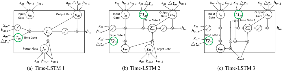
This version adds one time gate Tm to LSTM, which is shown in Fig. 2 (a). Based on the update equations (Eq. (1)∼(5)) of LSTM, we add one update equation for Tm as:
We then modify Eq. (3) and Eq. (4) to:
△tm is the time interval and σ△t is a sigmoid function. Tm is helpful in two ways. As shown in Eq. (13), on one hand, σc(xmWxc +hm-1Whc +bc) is filtered by not only the input gate im, but also the time gate Tm. So Tm can control the influence of xm on current recommendations. On the other hand, △tm is firstly stored in Tm, then transferred to cm, and would be transferred to cm+1, cm+2 · · · . Thus Tm helps to store △tm to model users' long-term interest (cm, cm+1 · · · ) for later recommendations. Note that, in a similar way, we are able to generalize Tm to other RNN architectures, such as GRU [Cho et al., 2014].
Tm is fully learned from data. However, as a priori knowledge, we know that given a certain last consumed item, if it is more recently consumed, it should have a larger influence on current recommendations. We want to incorporate this priori knowledge into the design of the time gate.
4.2 Time-LSTM2
Two time gates, i.e. T1m and T2m, are designed in this version. T1m is to control the influence of the last consumed item on current item recommendations, and T2m is to store time intervals to model users' long-term interest for later recommendations. The architecture is shown in Fig. 2 (b). Based on the update equations of LSTM, we first add two update equations for T1m and T2m as:
We then modify Eq. (3)∼(5) to:
om = σo(xmWxo
+ △tmWto + hm-1Who + wco ⊙ ˜
cm + bo),
(19)
Just as the input gate im in Eq. (17), T1m can be regarded as another filter, so that σc(xmWxc + hm-1Whc + bc) is filtered by not only im but also T1m. We use a new cell state ˜ cm to store the result, which is then transferred to the output gate om, the hidden state hm and finally influences current item recommendations. T2m firstly stores △tm, then transfers it to cm, and would transfer it to cm+1, cm+2 · · · to model users' long-term interest for later recommendations. Thus in Eq. (18), T2m acts more as the role of σc(xmWxc + hm-1Whc + bc).
Through the constraint Wt1 ≤ 0 in Eq. (15), T1m can exploit the priori knowledge described in section 4.1 to control the influence of xm on current item recommendations. Specifically, if △tm is smaller, according to Eq. (15), T1m would be larger. Then according to Eq. (17), xm would have a larger influence on current item recommendations (i.e. xm better reflects the short-term interest, thus we increase its influence). On the other hand, if △tm is larger, with a similar analysis, xm would have a smaller influence and correspondingly cm-1 would more significantly affect current recommendations (i.e. we are more uncertain about the short-term interest, thus we increase the influence of the long-term interest). For T2m, however, it doesn't make sense to impose such constraint on Wt2 in Eq. (16) in terms of modeling users' long-term interest for later recommendations. This also explains why we design two time gates in this version, i.e. to distinguish and customize the role for current recommendations and the role for later recommendations.
4.3 Time-LSTM3
Inspired by [Greff et al., 2016], this version (Fig. 2 (c)) uses coupled input and forget gates. Specifically, based on TimeLSTM 2, we remove the forget gate, and modify Eq. (17) and Eq. (18) to:
Since T1m is regarded as a filter (similar to im), thus we replace the forget gate with (1-im⊙T1m) in Eq. (21). T2m is to store time intervals (similar to σc(xmWxc + hm-1Whc + bc)), thus we use (1-im) in Eq. (22). The difference between Time-LSTM 3 and [Greff et al., 2016] lies in that (1) time gates exist in Time-LSTM 3 but not in [Greff et al., 2016] and, (2) Time-LSTM 3 has one additional coupled gate and one additional cell state.
The way we adapt Time-LSTM to our task is similar to the second way of LSTM's adaptations. Firstly, we transform Hu to [(iu1 , tu2 -tu1 ), (iu2 , tu3 -tu2 ), · · · , (iunu , tq -tunu )]. Then xm in Time-LSTM is equivalent to ium in our task. △tm is equivalent to tum+1 - tum.
4.4 Training
The parameters in Time-LSTM models are optimized by AdaGrad [Duchi et al., 2011], a variant of Stochastic Gradient Descent (SGD). For the constraint Wt1 ≤ 0 in Eq. (15), we use the projection operator described in [Rakhlin et al., 2012] to handle it, i.e. if we have Wt1 > 0 during training iterations, we reset Wt1 = 0.
In real-world applications, users' new consuming actions are continually generated. Other users' consuming histories help to provide "collaborative information" for the target user's recommendations. Meanwhile, this user's previous consuming history can provide "personalized information" for his later recommendations. Thus we want to make use of all available consuming histories (including newly generated actions) for recommendations, i.e. an online learning setting [Zhao et al., 2016]. To achieve this, we adapt the dynamic updated model in [Mikolov et al., 2010] to our task as follows. Step one, our model is trained on users' existing consuming histories until convergence. Step two, we repeat following procedure: After n (increase n for efficiency) new actions being generated, we update previous parameters once by applying AdaGrad to users' updated consuming histories. We may repeat above two steps periodically. The period can be tuned considering both of the recommendation performance and computational cost.
5 Experiments
5.1 Datasets and Experiment Settings
Our proposed algorithm is evaluated on two datasets, LastFM 1 and CiteULike 2 . For the LastFM dataset, we extract tuples <user id, song id, timestamp>, where each represents the action that user user id listens to song song id at time timestamp. For the CiteULike dataset, one user annotating one research paper at a certain time may have several records, in order to distinguish different tags. We merge them as one record and extract tuples <user id, paper id, timestamp>. Note that different from works such as [Zhu et al., 2016], tags are not exploited for recommendations in this paper. Users and items with few interactions are filtered. These tuples are organized by user id and ordered by timestamp. Table 1 shows their statistics.
For each dataset, 80% users are randomly selected as training users and their tuples are used for training. The remaining users are test users. For each test user u, its ordered tuples T u := [(u, iu1 , tu1 ), (u, iu2 , tu2 ), · · · , (u, iun′u , tun′u )] would generate n′u - 1 test cases, where the k-th test case is to perform recommendations at time tuk+1 given u's consuming history [(iu1 , tu1 ), (iu2 , tu2 ), · · · , (iuk , tuk )] with the ground truth iuk+1 .
5.2 ComparedMethods
We compare Time-LSTM to the following methods. The method in [Yu et al., 2016] is not compared, because its setting is different from ours and some techniques, e.g. pooling operations, cannot be applied to our task.
1 http://www.dtic.upf.edu/∼ocelma/MusicRecommendationDataset /lastfm-1K.html
2 http://www.citeulike.org/faq/data.adp
| LastFM | CiteULike | |
|---|---|---|
| Number of Users | 987 | 1625 |
| Number of Items | 5000 | 5000 |
| Number of Actions | 818767 | 35934 |
CoOccur+BPR: This is a combining strategy proposed in [Jannach et al., 2015], where CoOccur is to capture the shortterm interest and BPR is to capture the long-term interest. Specifically, CoOccur ranks items by the conditional probability of item co-occurring in users' sessions (association rules). Other items are appended to the recommendation list (if it is not filled up yet) ranked by BPR. We do not use FeatureMatching and RecentlyViewed in [Jannach et al., 2015]. The reason is that, FeatureMatching requires items' attribute information, which is not available in our task. RecentlyViewed simply recommends recently viewed items. However, in most cases, we want the RS to provide us with favorable items that we ignore, since even without the help of RS, we can still find items that we are familiar with (e.g. items that we recently viewed or comsumed). This method needs the session information. We use a commonly used approach, timeout [Huang et al., 2004], to identify sessions in users' consuming histories.
Session-RNN: This method [Hidasi et al., 2016a] uses RNN to capture the short-term interest based on items within a session in session-based recommendations. The long-term interest is not considered. The session information is extracted as described in CoOccur+BPR. We use the publicly available python implementation 3 of Session-RNN.
LSTM: The first way of LSTM's adaptation in section 3.2. LSTM+time: The second way of LSTM's adaptation in section 3.2.
Phased LSTM: Phased LSTM's adaptation in section 3.2.
The dynamic updated model described in section 4.4 is applied to LSTM and its variants, where the tuples of training users are used to train the model for step one. A similar updating strategy is applied to CoOccur+BPR and Session-RNN to ensure fair comparisons. The number of units is set to 512 for LSTM and its variants. The other hyperparameters in all methods are tuned via cross-validation or set as in the original paper. Our code is publicly available 4 .
5.3 Evaluations
Recall@10: Each target item ig (ground truth) is combined with 100 other random items. These 101 items are then ranked by the method and the top 10 items form the recommendation list. Recall@10 is defined as:
nhit is the number of test cases where ig is in the recommendation list and ntestcase is the number of all test cases. MRR@10 (Mean Reciprocal Rank): This is the average of reciprocal ranks of ig in the recommendation list. The reciprocal rank is set to 0 if the rank is above 10. MRR@10 takes into account the rank of the item.
3 https://github.com/hidasib/GRU4Rec
4 https://github.com/DarryO/time lstm
Each metric is evaluated 10 times and averaged. These two metrics are also used in [Jannach et al., 2015].
5.4 Results and Discussions
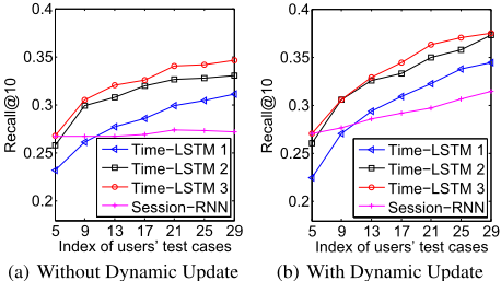
Method Comparison: As shown in Table 2, Time-LSTM models generally outperform other baselines. Time-LSTM 2 and Time-LSTM 3 have better performance than Time-LSTM 1, which demonstrates the effectiveness of using two time gates instead of one time gate. T 1m = 1 and T 2m = 1 are the results when we rewrite Eq. (15) to T1m = 1 and Eq. (16) to T2m = 1, respectively. They perform worse than the original version, which indicates that using our designed T1m to filter the input and T2m to store time intervals can both improve the performance. LSTM+time performs slightly worse than LSTM in CiteULike, which may be due to the usually large time intervals in CiteULike (after normalization, its performance improves, but is still worse than Time-LSTMmodels). Performance on Cold and Warm Users: We regard users as cold if they have consumed few items and warm if the opposite. Due to space limitation, we only show the results of Recall@10 in LastFM. As shown in Figure 3, the index k in the x-axis represents the k-th test cases, where we predict test users' (k + 1)-th actions given all the actions of training users and the first k actions of test users. (a) demonstrates that Time-LSTM performs better for warm users (larger indexes indicate that users have consumed more items). The reason is that with more actions contained in cm-1, Time-LSTM can better model the long-term interest for recommendations. For cold users, the performance of Time-LSTM is comparable to that of Session-RNN. This is because that although with few consuming actions, Time-LSTM can still well perform recommendations by capturing the short-term interest. The performance in (b) is better than that in (a), which proves the effectiveness of the dynamic updated model. The performance improvement from (a) to (b) is more remarkable for warm users, because the model is updated more times when users are warm than when they are cold.
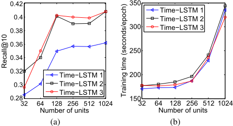
Number of Units and Efficiency: We vary the number of units (nu) to see how the performance and training time change. The training time is evaluated on a GeForce GTX Titan Black GPU. Due to space limitation, we only show the results of Recall@10 and the training time in LastFM. As shown in Figure 4 (a), increasing nu can improve Recall@10, but the improvement slows down or it even deteriorates when nu is larger than 128. On the other hand, as shown in Figure 4 (b), the training time is continually increasing when nu varies, and it is expensive to move from 512 units to 1024. Thus it is appropriate to assign [128, 512] to nu. Time-LSTM 3 always has a less training time than Time-LSTM 2 when nu varies. The reason is that the coupled input and forget gates in Time-LSTM 3 reduce the number of parameters and speed up the training process.
6 Conclusions
We propose Time-LSTM to model users' sequential actions in RS, where time intervals between neighbour actions are modeled by time gates in Time-LSTM. We design three versions of Time-LSTM, which well capture users' short-term and long-term interests at the same time, so as to improve the recommendation performance. Experimental results on two real-world datasets also show the effectiveness of TimeLSTM. In future work, we would design new versions of Time-LSTM to simultaneously model different types of behaviors in other application scenarios, e.g. click/collect/addto-cart/pay-for in e-commerce platforms. In addition, our method cannot generate recommendations for users who have no actions. Inspired by [Wang et al., 2016a; 2016b], we will explore the active learning solutions to this issue.
| LastFM | CiteULike | ||||
|---|---|---|---|---|---|
| Recall@10 | MRR@10 | Recall@10 | MRR@10 | ||
| CoOccur+BPR | 0.3217 | 0.1401 | 0.6954 | 0.2901 | |
| Session-RNN | 0.3405 | 0.1573 | 0.7129 | 0.2997 | |
| LSTM | 0.2451 | 0.0892 | 0.6824 | 0.2889 | |
| LSTM+time | 0.2628 | 0.0977 | 0.6655 | 0.2831 | |
| Phased LSTM | 0.2360 | 0.0859 | 0.6087 | 0.2539 | |
| Time-LSTM 1 | 0.3566 | 0.1853 | 0.7428 | 0.3179 | |
| Time-LSTM 2 | original | 0.3909 | 0.2250 | 0.7476 | 0.3377 |
| T 1m = 1 | 0.3236 | 0.1812 | 0.7058 | 0.3044 | |
| T 2m = 1 | 0.3643 | 0.2073 | 0.7014 | 0.3105 | |
| original | 0.3990 | 0.2657 | 0.7585 | 0.3660 | |
| Time-LSTM 3 T 1m = 1 | 0.3742 | 0.2212 | 0.6874 | 0.3046 | |
| T 2m = 1 | 0.3677 | 0.2249 | 0.7128 | 0.3232 | |
Acknowledgements
This work was supported by the National Basic Research Program of China (973 Program) under Grant 2013CB336500 and National Natural Science Foundation of China under Grant 61672409, 61379071, 61522206, 61373118. Also thanks to Prof. Xifeng Yan and his students in UCSB.
@inproceedings{ijcai2017p504,
  title     = {What to Do Next: Modeling User Behaviors by Time-LSTM},
  author    = {Zhu, Yu and Li, Hao and Liao, Yikang and Wang, Beidou and Guan, Ziyu and Liu, Haifeng and Cai, Deng},
  booktitle = {Proceedings of the Twenty-Sixth International Joint Conference on
               Artificial Intelligence, {IJCAI-17}},
  publisher = {International Joint Conferences on Artificial Intelligence Organization},
  editor    = {Carles Sierra},
  pages     = {3602--3608},
  year      = {2017},
  month     = {8},
  note      = {Main track},
  doi       = {10.24963/ijcai.2017/504},
  url       = {https://doi.org/10.24963/ijcai.2017/504},
}
TY - CPAPER TI - What to Do Next: Modeling User Behaviors by Time-LSTM AU - Zhu, Yu AU - Li, Hao AU - Liao, Yikang AU - Wang, Beidou AU - Guan, Ziyu AU - Liu, Haifeng AU - Cai, Deng T2 - Proceedings of the Twenty-Sixth International Joint Conference on Artificial Intelligence, IJCAI-17 PB - International Joint Conferences on Artificial Intelligence Organization PY - 2017 SP - 3602 EP - 3608 DO - 10.24963/ijcai.2017/504 UR - https://doi.org/10.24963/ijcai.2017/504 ER -Copied
Machine-readable versions of this paper, for tools and AI agents:





