
RAFT: Recurrent All-Pairs Field Transforms for Optical Flow (Extended Abstract)
Proceedings of the Thirtieth International Joint Conference on Artificial Intelligence. Sister Conferences Best Papers. Pages 4839-4843.
https://doi.org/10.24963/ijcai.2021/662
Keywords
- Computer Vision: 2D and 3D Computer Vision
- Computer Vision: Motion and Tracking
Abstract
We introduce Recurrent All-Pairs Field Transforms (RAFT), a new deep network architecture for optical flow. RAFT extracts per-pixel features, builds multi-scale 4D correlation volumes for all pairs of pixels, and iteratively updates a flow field through a recurrent unit that performs lookups on the correlation volumes. RAFT achieves state-of-the-art performance on the KITTI and Sintel datasets. In addition, RAFT has strong cross-dataset generalization as well as high efficiency in inference time, training speed, and parameter count.
- [Adler and Öktem, 2017] Jonas Adler and Ozan Öktem. Solving ill-posed inverse problems using iterative deep neural networks. Inverse Problems, 33(12):124007, 2017.
- [Amos and Kolter, 2017] Brandon Amos and J Zico Kolter. Opt- net: Differentiable optimization as a layer in neural networks. In Proceedings of the 34th International Conference on Machine Learning-Volume 70, pages 136-145. JMLR. org, 2017.
- [Bar-Haim and Wolf, 2020] Aviram Bar-Haim and Lior Wolf. Scopeflow: Dynamic scene scoping for optical flow. In Pro- ceedings of the IEEE/CVF Conference on Computer Vision and Pattern Recognition, pages 7998-8007, 2020.
- [Black and Anandan, 1993] Michael J Black and Padmanabhan Anandan. A framework for the robust estimation of optical flow. In 1993 (4th) International Conference on Computer Vi- sion, pages 231-236. IEEE, 1993.
- [Brox et al., 2009] Thomas Brox, Christoph Bregler, and Jitendra Malik. Large displacement optical flow. In 2009 IEEE Confer- ence on Computer Vision and Pattern Recognition, pages 41-48. IEEE, 2009.
- [Butler et al., 2012] Daniel J Butler, Jonas Wulff, Garrett B Stanley, and Michael J Black. A naturalistic open source movie for opti- cal flow evaluation. In European conference on computer vision, pages 611-625. Springer, 2012.
- [Chambolle and Pock, 2011] Antonin Chambolle and Thomas Pock. A first-order primal-dual algorithm for convex problems with applications to imaging. Journal of mathematical imaging and vision, 40(1):120-145, 2011.
- [Dosovitskiy et al., 2015] Alexey Dosovitskiy, Philipp Fischer, Eddy Ilg, Philip Hausser, Caner Hazirbas, Vladimir Golkov, Patrick Van Der Smagt, Daniel Cremers, and Thomas Brox. Flownet: Learning optical flow with convolutional networks. In Proceedings of the IEEE international conference on computer vision, pages 2758-2766, 2015.
- [Hofinger et al., 2020] Markus Hofinger, Samuel Rota Bulò, Lorenzo Porzi, Arno Knapitsch, and Peter Kontschieder. Improv- ing optical flow on a pyramidal level. In ECCV, 2020.
- [Horn and Schunck, 1981] Berthold KP Horn and Brian G Schunck. Determining optical flow. In Techniques and Appli- cations of Image Understanding, volume 281, pages 319-331. International Society for Optics and Photonics, 1981.
- [Hur and Roth, 2019] Junhwa Hur and Stefan Roth. Iterative resid- ual refinement for joint optical flow and occlusion estimation. In Proceedings of the IEEE Conference on Computer Vision and Pattern Recognition, pages 5754-5763, 2019.
- [Ilg et al., 2017] Eddy Ilg, Nikolaus Mayer, Tonmoy Saikia, Mar- gret Keuper, Alexey Dosovitskiy, and Thomas Brox. Flownet 2.0: Evolution of optical flow estimation with deep networks. In Proceedings of the IEEE conference on computer vision and pat- tern recognition, pages 2462-2470, 2017.
- [Kondermann et al., 2016] Daniel Kondermann, Rahul Nair, Ka- trin Honauer, Karsten Krispin, Jonas Andrulis, Alexander Brock, Burkhard Gussefeld, Mohsen Rahimimoghaddam, Sabine Hof- mann, Claus Brenner, et al. The hci benchmark suite: Stereo and flow ground truth with uncertainties for urban autonomous driv- ing. In Proceedings of the IEEE Conference on Computer Vision and Pattern Recognition Workshops, pages 19-28, 2016.
- [Loshchilov and Hutter, 2018] Ilya Loshchilov and Frank Hutter. Decoupled weight decay regularization. In International Con- ference on Learning Representations, 2018.
- [Lu et al., 2020] Yao Lu, Jack Valmadre, Heng Wang, Juho Kan- nala, Mehrtash Harandi, and Philip Torr. Devon: Deformable volume network for learning optical flow. In The IEEE Winter Conference on Applications of Computer Vision, 2020.
- [Mayer et al., 2016] Nikolaus Mayer, Eddy Ilg, Philip Hausser, Philipp Fischer, Daniel Cremers, Alexey Dosovitskiy, and Thomas Brox. A large dataset to train convolutional networks for disparity, optical flow, and scene flow estimation. In Proceed- ings of the IEEE Conference on Computer Vision and Pattern Recognition, pages 4040-4048, 2016.
- [Menze and Geiger, 2015] Moritz Menze and Andreas Geiger. Ob- ject scene flow for autonomous vehicles. In Proceedings of the IEEE conference on computer vision and pattern recognition, pages 3061-3070, 2015.
- [Paszke et al., 2019] Adam Paszke, Sam Gross, Francisco Massa, Adam Lerer, James Bradbury, Gregory Chanan, Trevor Killeen, Zeming Lin, Natalia Gimelshein, Luca Antiga, Alban Desmai- son, Andreas Kopf, Edward Yang, Zachary DeVito, Martin Raison, Alykhan Tejani, Sasank Chilamkurthy, Benoit Steiner, Lu Fang, Junjie Bai, and Soumith Chintala. Pytorch: An impera- tive style, high-performance deep learning library. In Advances in Neural Information Processing Systems, pages 8024-8035. 2019.
- [Ranftl et al., 2014] René Ranftl, Kristian Bredies, and Thomas Pock. Non-local total generalized variation for optical flow es- timation. In European Conference on Computer Vision, pages 439-454. Springer, 2014.
- [Ranjan and Black, 2017] Anurag Ranjan and Michael J Black. Op- tical flow estimation using a spatial pyramid network. In Pro- ceedings of the IEEE Conference on Computer Vision and Pat- tern Recognition, pages 4161-4170, 2017.
- [Sun et al., 2018a] Deqing Sun, Xiaodong Yang, Ming-Yu Liu, and Jan Kautz. Models matter, so does training: An empiri- cal study of cnns for optical flow estimation. arXiv preprint arXiv:1809.05571, 2018.
- [Sun et al., 2018b] Deqing Sun, Xiaodong Yang, Ming-Yu Liu, and Jan Kautz. Pwc-net: Cnns for optical flow using pyramid, warp- ing, and cost volume. In Proceedings of the IEEE Conference on Computer Vision and Pattern Recognition, pages 8934-8943, 2018.
- [Tang and Tan, 2018] Chengzhou Tang and Ping Tan. Ba- net: Dense bundle adjustment network. arXiv preprint arXiv:1806.04807, 2018.
- [Weinzaepfel et al., 2013] Philippe Weinzaepfel, Jerome Revaud, Zaid Harchaoui, and Cordelia Schmid. Deepflow: Large dis- placement optical flow with deep matching. In Proceedings of the IEEE international conference on computer vision, pages 1385- 1392, 2013.
- [Yang and Ramanan, 2019] Gengshan Yang and Deva Ramanan. Volumetric correspondence networks for optical flow. In Ad- vances in Neural Information Processing Systems, pages 793- 803, 2019.
- [Zach et al., 2007] Christopher Zach, Thomas Pock, and Horst Bischof. A duality based approach for realtime tv-l 1 optical flow. In Joint pattern recognition symposium, pages 214-223. Springer, 2007.
- [Zhao et al., 2020] Shengyu Zhao, Yilun Sheng, Yue Dong, Eric I Chang, Yan Xu, et al. Maskflownet: Asymmetric feature matching with learnable occlusion mask. In Proceedings of the IEEE/CVF Conference on Computer Vision and Pattern Recog- nition, pages 6278-6287, 2020.
References were extracted automatically from the PDF and may contain errors.
Full text extracted automatically from the PDF; figures, tables and equations may differ. The PDF is the version of record.
1 Introduction
Optical flow is the task of estimating per-pixel motion between video frames. It is a long-standing vision problem that remains unsolved. The best systems are limited by difficulties including fast-moving objects, occlusions, motion blur, and textureless surfaces.
Optical flow has traditionally been approached as a handcrafted optimization problem over the space of dense displacement fields between a pair of images [Horn and Schunck, 1981]. Generally, the optimization objective defines a trade-off between a data term which encourages the alignment of visually similar image regions and a regularization term which imposes priors on the plausibility of motion. Such an approach has achieved considerable success, but further progress has appeared challenging, due to the difficulties in hand-designing an optimization objective that is robust to a variety of corner cases.
Recently, deep learning has been shown as a promising alternative to traditional methods. Deep learning can sidestep formulating an optimization problem and train a network to directly predict flow. Current deep learning methods[Ilg et al., 2017; Sun et al., 2018b; Yang and Ramanan, 2019; Hofinger et al., 2020] have achieved performance comparable to the best traditional methods while being significantly faster at inference time. A key question for further research is designing effective architectures that perform better, train more easily and generalize well to novel scenes.
We introduce Recurrent All-Pairs Field Transforms (RAFT), a new deep network architecture for optical flow. RAFT enjoys the following strengths:
- State-of-the-art accuracy: On KITTI [Menze and Geiger, 2015], RAFT achieves an F1-all error of 5.10%, a 16% error reduction from the best published result (6.10%). On Sintel [Butler et al., 2012] (final pass), RAFT obtains an end-point-error of 2.86 pixels, a 30% error reduction from the best published result.
- Strong generalization: When trained only on synthetic data, RAFT achieves an end-point-error of 5.04 pixels on KITTI [Menze and Geiger, 2015], a 40% error reduction from the best prior approach.
- High efficiency: RAFT processes 1088 × 436 videos at 10 frames per second on a 1080Ti GPU. It trains with 10X fewer iterations than other architectures. A smaller version of RAFT runs at 20fps.
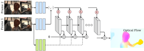
RAFT consists of three main components: (1) a feature encoder that extracts a feature vector for each pixel; (2) a correlation layer that produces a 4D correlation volume for all pairs of pixels, with subsequent pooling to produce lower resolution volumes; (3) a recurrent GRU-based update operator that retrieves values from the correlation volumes and iteratively updates a flow field initialized at zero (Fig. 1).
The RAFT architecture is motivated by traditional optimization-based approaches. The feature encoder extracts per-pixel features. The correlation layer computes visual similarity between pixels. The update operator mimics the steps of an iterative optimization algorithm. But unlike traditional approaches, features and motion priors are not handcrafted but learned-learned by the feature encoder and the update operator respectively.
The design of RAFT draws inspiration from many existing works but is substantially novel. First, RAFT maintains and updates a single fixed flow field at high resolution. This is different from the prevailing coarse-to-fine design in prior work [Sun et al., 2018b; Yang and Ramanan, 2019; Hur and Roth, 2019], where flow is first estimated at low resolution and upsampled and refined at high resolution. By operating on a single high-resolution flow field, RAFT overcomes several limitations of a coarse-to-fine cascade: the difficulty of recovering from errors at coarse resolutions, the tendency to miss small fast-moving objects.
Second, the update operator has a novel design. Guided by first order optimization algorithms, we design an update operator which is recurrent and lightweight. It consists of a convolutional GRU that performs lookups on 4D multi-scale correlation volumes. During inference, the update operator uses correlation features make iterative updates to the flow field and can be applied 100+ times without divergence.
We conduct experiments on Sintel[Butler et al., 2012] and KITTI[Menze and Geiger, 2015]. Results show that RAFT achieves state-of-the-art performance on both datasets. In addition, we validate various design choices of RAFT through extensive ablation studies.
2 RelatedWork
2.1 Optical Flow as EnergyMinimization
Optical flow has traditionally been treated as an energy minimization problem which imposes a tradeoff between a data term and a regularization term. [Horn and Schunck, 1981] formulated optical flow as a continuous optimization problem using a variational framework, and were able to estimate a dense flow field by performing gradient steps. [Black and Anandan, 1993] addressed problems with oversmoothing and noise sensitivity by introducing a robust estimation framework. TV-L1 [Zach et al., 2007] replaced the quadratic penalties with an L1 data term and total variation regularization, which allowed for motion discontinuities and was better equipped to handle outliers. Improvements have been made by defining better matching costs [Weinzaepfel et al., 2013; Brox et al., 2009] and regularization [Ranftl et al., 2014].
Such continuous formulations maintain a single estimate of optical flow which is refined at each iteration. To ensure a smooth objective function, a first order Taylor approximation is used to model the data term. As a result, they only work well for small displacements. To handle large displacements, the coarse-to-fine strategy is used, where an image pyramid is used to estimate large displacements at low resolution, then small displacements refined at high resolution. But this coarse-to-fine strategy may miss small fast-moving objects and have difficulty recovering from early mistakes. Like continuous methods, we maintain a single estimate of optical flow which is refined with each iteration. However, since we build correlation volumes for all pairs at both high resolution and low resolution, each local update uses information about both small and large displacements.
2.2 Deep Learning for Optical Flow
Neural networks have been trained to directly predict optical flow between a pair of frames, side-stepping the optimization problem completely. Coarse-to-fine processing has emerged as a popular ingredient in many recent works [Sun et al., 2018b; Hur and Roth, 2019; Yang and Ramanan, 2019; Hofinger et al., 2020; Bar-Haim and Wolf, 2020; Zhao et al., 2020]. In contrast, our method maintains and updates a single high-resolution prediction of the optical flow field.
Many recent works have used iterative refinement to improve results on optical flow [Ilg et al., 2017; Ranjan and Black, 2017; Sun et al., 2018b; Yang and Ramanan, 2019]. [Ilg et al., 2017] applied iterative refinement to optical flow by stacking multiple FlowNetS and FlowNetC modules in series. SpyNet[Ranjan and Black, 2017], PWC-Net[Sun et al., 2018b], and VCN [Yang and Ramanan, 2019] apply iterative refinement using coarse-to-fine pyramids.
More closely related to our approach is IRR[Hur and Roth, 2019], which builds off of the FlownetS and PWC-Net architecture but shares weights between refinement networks. When using FlowNetS, it is limited by the size of the network (38M parameters) and is only applied up to 5 iterations. When using PWC-Net, iterations are limited by the number of pyramid levels. In contrast, we use a much simpler refinement module (2.7M parameters) which can be applied for 100+ iterations during inference without divergence. Our method also shares similarites with Devon [Lu et al., 2020], namely the construction of the cost volume without warping and fixed resolution updates. However, Devon does not have any recurrent unit nor a full correlation volume, and is limited to 3 refinement steps.
2.3 Learning to Optimize
Many problems in vision can be formulated as an optimization problem. This has motivated several works to embed optimization problems into network architectures [Amos and Kolter, 2017; Tang and Tan, 2018]. These works typically use a network to predict the inputs or parameters of the optimization problem, and then train the network weights by backpropogating the gradient through the solver, either implicitly[Amos and Kolter, 2017] or unrolling each step [Tang and Tan, 2018]. However, this technique is limited to problems with an easily defined objective.
Another approach is to learn iterative updates directly from data [Adler and ¨Oktem, 2017]. These approaches are motivated by the fact that first order optimizers such as Primal Dual Hybrid Gradient (PDHG)[Chambolle and Pock, 2011] can be expressed as a sequence of iterative update steps. Instead of using an optimizer directly, [Adler and ¨Oktem, 2017] proposed building a network which mimics the updates of a first order algorithm.
Our approach can be viewed as learning to optimize: our network uses a large number of update blocks to emulate the steps of a first-order optimization algorithm. However, unlike prior work, we never explicitly define a gradient with respect to some optimization objective. Instead, our network retrieves features from correlation volumes to propose the descent direction.
3 Approach
Given a pair of consecutive RGB images, I1, I2, we estimate a dense displacement field (f 1 , f 2 ) which maps each pixel (u, v) in I2 to its corresponding coordinates (u′ , v′ ) in I2. An overview of our approach is given in Figure 1. Our method can be distilled down to three stages: (1) feature extraction, (2) computing visual similarity, and (3) iterative updates, where all stages are differentiable and composed into an end-to-end trainable architecture.
3.1 Feature Extraction and Correlation Volume
Features are extracted from the input images using a convolutional network. The feature encoder network is applied to both I1 and I2 and maps the input images to dense feature maps at a lower resolution. Our encoder, gθ outputs features at 1/8 resolution gθ : RH×W×3 ↦→ RH/8×W/8×D with D = 256. The feature encoder consists of 6 residual blocks.
We additionally use a context network. The context network extracts features only from the first input image I1. The architecture of the context network, hθ is identical to the feature extraction network. Together, the feature network gθ and the context network hθ form the first stage of our approach, which only need to be performed once.
Computing Visual Similarity. We compute visual similarity by constructing a full correlation volume between all pairs. Given image features gθ(I1) ∈ RH×W×D and gθ(I2) ∈ RH×W×D , the correlation volume is formed by taking the dot product between all pairs of feature vectors. The correlation volume, C, can be efficiently computed as a single matrix multiplication.Cijkl = ∑
Correlation Volume. We construct a 4-layer pyramid {C1 ,C2 ,C3 ,C4 } by pooling the last two dimensions of the correlation volume with kernel sizes 1, 2, 4, and 8 and equivalent stride. Thus, volume Ck has dimensions H × W × H/2k ×W/2k . The set of volumes gives information about both large and small displacements; however, by maintaining the first 2 dimensions (the I1 dimensions) we maintain high resolution information, allowing our method to recover the motions of small fast-moving objects.
Correlation Lookup. We define a lookup operator LC which generates a feature map by indexing from the correlation pyramid. Given a current estimate of optical flow (f 1 , f 2 ), we map each pixel x = (u, v) in I1 to its estimated correspondence in I2: x′ = (u+f 1 (u), v +f 2 (v)). We then define a local grid around x′
as the set of integer offsets which are within a radius of r units of x′ using the L1 distance. We use the local neighborhood N(x′ )r to index from the correlation volume.
We perform lookups on all levels of the pyramid and concatenate the results. A constant radius across levels means larger context at lower levels; such that, as the lowest level, the neighborhood covers a 576x576 grid of pixels.
3.2 Update Operator
Our update operator estimates a sequence of flow estimates {f1, ..., fN} from an initial starting point f0 = 0. With each iteration, it produces an update direction ∆f which is applied to the current estimate: fk+1 = ∆f + fk.
The update operator takes flow, correlation, and a latent hidden state as input, and outputs the update ∆f and an updated hidden state. The architecture of our update operator is designed to mimic the steps of an optimization algorithm. As such, we used tied weights across depth and use bounded activations to encourage convergence to a fixed point. The update operator is trained to perform updates such that the sequence converges to a fixed point fk → f ∗ .
Initialization. By default, we initialize the flow field to 0 everywhere, but our iterative approach gives us the flexibility to experiment with alternatives. When applied to video, we test warm-start initialization, where optical flow from the previous pair of frames is forward projected to the next pair of frames with occlusion gaps interpolated.
Inputs. Given the current flow estimate f k , we use it to retrieve correlation features from the correlation pyramid. The correlation features are then processed by 2 convolutional layers. Additionally, we apply 2 convolutional layers to the flow estimate itself to generate flow features. Finally, we directly inject the input from the context network. The input feature map is then taken as the concatenation of the correlation, flow, and context features.
Update. Acore component of the update operator is a gated activation unit based on the GRU cell, with linear layers replaced with convolutions. Each iteration of the GRU takes in a state variable, which is the concatenation of flow, correlation, and context features. We also experiment with a separable ConvGRU unit, where we replace the 3 × 3 convolution with two GRUs: one with a 1 × 5 convolution and one with a 5 × 1 convolution to increase the receptive field without significantly increasing the size of the model.
Flow Prediction. The hidden state outputted by the GRU is passed through two convolutional layers to predict the flow update ∆f . The output flow is at 1/8 resolution of the input image. During training and evaluation, we upsample the predicted flow fields to match the resolution of the ground truth.
Upsampling. The network outputs optical flow at 1/8 resolution. We upsample the optical flow to full resolution by taking the full resolution flow at each pixel to be the convex combination of a 3x3 grid of its coarse resolution neighbors. We use two convolutional layers to predict a H/8 × W/8 × (8 × 8 × 9) mask and perform softmax over the weights of the 9 neighbors. The final high resolution flow field is found taking a weighted combination over the neighborhood, then reshaped to a full resolution flow field.
3.3 Supervision
We supervised our network on the l1 distance between the predicted and ground truth flow over the full sequence of predictions, {f1, ..., fN}, with exponentially increasing weights.
| Training Data | Method | Sintel (train) | KITTI-15 (train) | Sintel (test) | KITTI-15 (test) | |||
|---|---|---|---|---|---|---|---|---|
| Clean | Final | F1-epe | F1-all | Clean | Final | F1-all | ||
| PWC-Net [Sun et al., 2018b] | 2.55 | 3.93 | 10.35 | 33.7 | - | - | - | |
| VCN [Yang and Ramanan, 2019] | 2.21 | 3.68 | 8.36 | 25.1 | - | - | - | |
| MaskFlowNet [Zhao et al., 2020] | 2.25 | 3.61 | - | 23.1 | - | - | - | |
| C + T FlowNet2 [Ilg et al., 2017] | 2.02 | 3.54 | 10.08 | 30.0 | 3.96 | 6.02 | - | |
| Ours (small) | 2.21 | 3.35 | 7.51 | 26.9 | - | - | - | |
| Ours (2-view) | 1.43 | 2.71 | 5.04 | 17.4 | - | - | - | |
| FlowNet2 [Ilg et al., 2017] | (1.45) | (2.01) | (2.30) | (6.8) | 4.16 | 5.74 | 11.48 | |
| IRR-PWC [Hur and Roth, 2019] | (1.92) | (2.51) | (1.63) | (5.3) | 3.84 | 4.58 | 7.65 | |
| C+T+S/K ScopeFlow [Bar-Haim and Wolf, 2020] | - | - | - | - | 3.59 | 4.10 | 6.82 | |
| Ours (2-view) | (0.77) | (1.20) | (0.64) | (1.5) | 2.08 | 3.41 | 5.27 | |
| PWC-Net+ [Sun et al., 2018a] | (1.71) | (2.34) | (1.50) | (5.3) | 3.45 | 4.60 | 7.72 | |
| VCN [Yang and Ramanan, 2019] | (1.66) | (2.24) | (1.16) | (4.1) | 2.81 | 4.40 | 6.30 | |
| MaskFlowNet [Zhao et al., 2020] | - | - | - | - | 2.52 | 4.17 | 6.10 | |
| C+T+S+K+H Ours (2-view) | (0.76) | (1.22) | (0.63) | (1.5) | 1.94 | 3.18 | 5.10 | |
| Ours (warm-start) | (0.77) | (1.27) | - | - | 1.61 | 2.86 | - | |
Given ground truth flow fgt, the loss is defined as
4 Experiments
We evaluate RAFT on Sintel [Butler et al., 2012] and KITTI [Menze and Geiger, 2015]. Following previous works, we pretrain our network on FlyingChairs[Dosovitskiy et al., 2015] and FlyingThings[Mayer et al., 2016], followed by dataset specific finetuning.
Implementation. RAFT is implemented in PyTorch [Paszke et al., 2019] and initialized with random weights. We train using the AdamW optimizer [Loshchilov and Hutter, 2018] and clip gradients to the range [-1, 1]. Unless otherwise noted, we evaluate after 32 flow updates on Sintel and 24 on KITTI. For every update, ∆f + fk, we only backpropgate the gradient through the ∆f branch, and zero the gradient through the fk branch as suggested by [Hofinger et al., 2020].
Training Schedule. We train RAFT using two 2080Ti GPUs. We pretrain on FlyingThings for 100k iterations with a batch size of 12, then train for 100k iterations on FlyingThings3D with a batch size of 6. We finetune on Sintel for another 100k by combining data from Sintel[Butler et al., 2012], KITTI-2015 [Menze and Geiger, 2015], and HD1K[Kondermann et al., 2016] similar to prior work [Zhao et al., 2020; Sun et al., 2018a]. Finally, we finetune on KITTI-2015 for an additionally 50k iterations using the weights from the model finetuned on Sintel. For comparison with prior work, we also include results from our model when finetuning only on Sintel and only on KITTI.
Sintel. We train using the FlyingChairs→FlyingThings schedule and then evaluate on the Sintel dataset using the train split for validation. Results are shown in Tab. 1, and organized based on the data used for training. C + T means that the models are trained on Chairs(C) and Things(T), +ft indicates finetuning on Sintel.
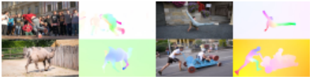
Our method ranks 1st on both the Sintel clean and final passes, and outperforms all prior work by 0.9 pixels (36%) on the clean pass and 1.2 pixels (30%) on the final pass. We evaluate two versions of our model, Ours (two-frame) uses zero initialization, while Ours (warp-start) initializes flow by forward projecting the flow estimate from the previous frame.
KITTI. We also evaluate RAFT on KITTI and provide results in Tab.1. We first evaluate cross-dataset generalization by evaluating on the KITTI-15 (train) split after training on Chairs(C) and FlyingThings(T). Our method outperforms prior works by a large margin, improving EPE (end-pointerror) from 8.36 to 5.04. Our method ranks 1st on the KITTI leaderboard among all optical flow methods.
5 Conclusions
We have proposed RAFT-Recurrent All-Pairs Field Transforms-a new end-to-end trainable model for optical flow. RAFT is unique in that it operates at a single resolution using a large number of lightweight, recurrent update operators. Our method achieves state-of-the-art accuracy across a diverse range of datasets, has strong cross dataset generalization, and is efficient in terms of inference time, parameter count, and training iterations.
@inproceedings{ijcai2021p662,
  title     = {RAFT: Recurrent All-Pairs Field Transforms for Optical Flow (Extended Abstract)},
  author    = {Teed, Zachary and Deng, Jia},
  booktitle = {Proceedings of the Thirtieth International Joint Conference on
               Artificial Intelligence, {IJCAI-21}},
  publisher = {International Joint Conferences on Artificial Intelligence Organization},
  editor    = {Zhi-Hua Zhou},
  pages     = {4839--4843},
  year      = {2021},
  month     = {8},
  note      = {Sister Conferences Best Papers},
  doi       = {10.24963/ijcai.2021/662},
  url       = {https://doi.org/10.24963/ijcai.2021/662},
}
TY - CPAPER TI - RAFT: Recurrent All-Pairs Field Transforms for Optical Flow (Extended Abstract) AU - Teed, Zachary AU - Deng, Jia T2 - Proceedings of the Thirtieth International Joint Conference on Artificial Intelligence, IJCAI-21 PB - International Joint Conferences on Artificial Intelligence Organization PY - 2021 SP - 4839 EP - 4843 DO - 10.24963/ijcai.2021/662 UR - https://doi.org/10.24963/ijcai.2021/662 ER -Copied
Machine-readable versions of this paper, for tools and AI agents:





