
CGS: Coupled Growth and Survival Model with Cohort Fairness
Proceedings of the Thirty-Second International Joint Conference on Artificial Intelligence. AI for Good. Pages 5986-5994.
https://doi.org/10.24963/ijcai.2023/664
Keywords
- AI for Good: Multidisciplinary Topics and Applications
- AI for Good: Data Mining
Abstract
Fish modeling in complex environments is critical for understanding drivers of population dynamics in aquatic systems. This paper proposes a Bayesian network method for modeling fish survival and growth over multiple connected rivers. Traditional fish survival models capture the effect of multiple environmental drivers (e.g., stream temperature, stream flow) by adding different variables, which increases model complexity and results in very long and impractical run times (i.e., weeks). We propose a coupled survival-growth model that leverages the observations from both sources simultaneously. It also integrates the Bayesian process into the neural network model to efficiently capture complex variable relationships in the system while also conforming to known survival processes used in existing fish models. To further reduce the performance disparity of fish body length across cohorts, we propose two approaches for enforcing fairness by the adjustment of training priorities and data augmentation. The results based on a real-world fish dataset collected in Massachusetts, US demonstrate that the proposed method can greatly improve prediction accuracy in modeling survival and body length compared to independent models on survival and growth, and effectively reduce the performance disparity across cohorts. The fish growth and movement patterns discovered by the proposed model are also consistent with prior studies in the same region, while vastly reducing run times and memory requirements.
- [Alasadi et al., 2019] Jamal Alasadi, Ahmed Al Hilli, and Vivek K Singh. Toward fairness in face matching algo- rithms. In Proceedings of the 1st International Workshop on Fairness, Accountability, and Transparency in Multi- Media, pages 19-25, 2019.
- [Belloni and Chernozhukov, 2009] Alexandre Belloni and Victor Chernozhukov. On the computational complexity of MCMC-based estimators in large samples. The Annals of Statistics, 37(4):2011 -2055, 2009.
- [Bonnaffé et al., 2021] Willem Bonnaffé, Ben C Sheldon, and Tim Coulson. Neural ordinary differential equations for ecological and evolutionary time-series analysis. Meth- ods in Ecology and Evolution, 12(7):1301-1315, 2021.
- [Coulson et al., 2011] Tim Coulson, Daniel R MacNulty, Daniel R Stahler, Bridgett VonHoldt, Robert K Wayne, and Douglas W Smith. Modeling effects of environmental change on wolf population dynamics, trait evolution, and life history. Science, 334(6060):1275-1278, 2011.
- [Grade and Letcher, 2006] Melissa Grade and Benjamin H Letcher. Diel and seasonal variation in food habits of at- lantic salmon parr in a small stream. Journal of Freshwater Ecology, 21(3):503-517, 2006.
- [He et al., 2022] Erhu He, Yiqun Xie, Xiaowei Jia, Weiye Chen, Han Bao, Xun Zhou, Zhe Jiang, Rahul Ghosh, and Praveen Ravirathinam. Sailing in the location-based fairness-bias sphere. In Proceedings of the 30th Interna- tional Conference on Advances in Geographic Information Systems, pages 1-10, 2022.
- [Heckerman, 1998] David Heckerman. A tutorial on learn- ing with Bayesian networks. Springer, 1998.
- [Hochreiter and Schmidhuber, 1997] Sepp Hochreiter and Jürgen Schmidhuber. Long short-term memory. Neural computation, 9(8):1735-1780, 1997.
- [Hopkins, 1992] Kevin D Hopkins. Reporting fish growth: A review of the basics 1. Journal of the world aquaculture society, 23(3):173-179, 1992.
- [Jang et al., 2016] Eric Jang, Shixiang Gu, and Ben Poole. Categorical reparameterization with gumbel-softmax. arXiv preprint arXiv:1611.01144, 2016.
- [Joseph, 2020] Maxwell B Joseph. Neural hierarchical mod- els of ecological populations. Ecology Letters, 23(4):734- 747, 2020.
- [Kamishima et al., 2011] Toshihiro Kamishima, Shotaro Akaho, and Jun Sakuma. Fairness-aware learning through regularization approach. In 2011 IEEE 11th International Conference on Data Mining Workshops, pages 643-650. IEEE, 2011.
- [Kanno et al., 2015] Yoichiro Kanno, Benjamin H Letcher, Nathaniel P Hitt, David A Boughton, John EB Wofford, and Elise F Zipkin. Seasonal weather patterns drive pop- ulation vital rates and persistence in a stream fish. Global Change Biology, 21(5):1856-1870, 2015.
- [Kingma and Welling, 2013] Diederik P Kingma and Max Welling. Auto-encoding variational bayes. arXiv preprint arXiv:1312.6114, 2013.
- [Letcher et al., 2005] Benjamin H Letcher, Gregg E Horton, Todd L Dubreuil, and Matthew J O'Donnell. A field test of the extent of bias in selection estimates after accounting for emigration. Evolutionary Ecology Research, 7(4):643- 650, 2005.
- [Letcher et al., 2015] Benjamin H Letcher, Paul Schueller, Ronald D Bassar, Keith H Nislow, Jason A Coombs, Krzysztof Sakrejda, Michael Morrissey, Douglas B Sigourney, Andrew R Whiteley, Matthew J O'Donnell, et al. Robust estimates of environmental effects on pop- ulation vital rates: an integrated capture-recapture model of seasonal brook trout growth, survival and movement in a stream network. Journal of Animal Ecology, 84(2):337- 352, 2015.
- [Lorenzen et al., 2022] Kai Lorenzen, Edward V Camp, and Taryn M Garlock. Natural mortality and body size in fish populations. Fisheries Research, 252:106327, 2022.
- [Mohankumar and Hefley, 2022] Narmadha M Mohanku- mar and Trevor J Hefley. Using machine learning to model nontraditional spatial dependence in occupancy data. Ecology, 103(2):e03563, 2022.
- [Ozgul et al., 2009] Arpat Ozgul, Shripad Tuljapurkar, Tim G Benton, Josephine M Pemberton, Tim H Clutton- Brock, and Tim Coulson. The dynamics of phenotypic change and the shrinking sheep of st. kilda. Science, 325(5939):464-467, 2009.
- [Pelletier et al., 2012] Fanie Pelletier, Kelly Moyes, Tim H Clutton-Brock, and Tim Coulson. Decomposing varia- tion in population growth into contributions from envi- ronment and phenotypes in an age-structured population. Proceedings of the Royal Society B: Biological Sciences, 279(1727):394-401, 2012.
- [Raabe et al., 2014] Joshua K Raabe, Beth Gardner, and Joseph E Hightower. A spatial capture-recapture model to estimate fish survival and location from linear continu- ous monitoring arrays. Canadian Journal of Fisheries and Aquatic Sciences, 71(1):120-130, 2014.
- [Royle, 2008] J Andrew Royle. Modeling individual effects in the cormack-jolly-seber model: a state-space formula- tion. Biometrics, 64(2):364-370, 2008.
- [Seo et al., 2021] Eugene Seo, Rebecca A Hutchinson, Xiao Fu, Chelsea Li, Tyler A Hallman, John Kilbride, and W Douglas Robinson. Stateconet: Statistical ecology neu- ral networks for species distribution modeling. In Pro- ceedings of the AAAI Conference on Artificial Intelligence, volume 35, pages 513-521, 2021.
- [Serna et al., 2022] Ignacio Serna, Aythami Morales, Julian Fierrez, and Nick Obradovich. Sensitive loss: Improv- ing accuracy and fairness of face representations with discrimination-aware deep learning. Artificial Intelligence, 305:103682, 2022.
- [Sigourney et al., 2008] DB Sigourney, BH Letcher, M Obedzinski, and RA Cunjak. Size-independent growth in fishes: patterns, models and metrics. Journal of Fish Biology, 72(10):2435-2455, 2008.
- [Sweeney and Najafian, 2020] Chris Sweeney and Maryam Najafian. Reducing sentiment polarity for demographic attributes in word embeddings using adversarial learning. In Proceedings of the 2020 Conference on Fairness, Ac- countability, and Transparency, pages 359-368, 2020.
- HG Washington. Diversity, biotic and similarity indices: a review with special relevance to aquatic ecosystems. Water research, 18(6):653-694, 1984.
- [Xie et al., 2021a] Yiqun Xie, Erhu He, Xiaowei Jia, Han Bao, Xun Zhou, Rahul Ghosh, and Praveen Ravirathi- nam. A statistically-guided deep network transformation and moderation framework for data with spatial hetero- geneity. In 2021 IEEE International Conference on Data Mining (ICDM), pages 767-776. IEEE, 2021.
- [Xie et al., 2021b] Yiqun Xie, Xiaowei Jia, Han Bao, Xun Zhou, Jia Yu, Rahul Ghosh, and Praveen Ravirathinam. Spatial-net: A self-adaptive and model-agnostic deep learning framework for spatially heterogeneous datasets. In Proceedings of the 29th International Conference on Advances in Geographic Information Systems, pages 313- 323, 2021.
- [Xie et al., 2022] Yiqun Xie, Erhu He, Xiaowei Jia, Weiye Chen, Sergii Skakun, Han Bao, Zhe Jiang, Rahul Ghosh, and Praveen Ravirathinam. Fairness by "where": A statistically-robust and model-agnostic bi-level learning framework. In Proceedings of the AAAI Conference on Ar- tificial Intelligence, volume 36, pages 12208-12216, 2022.
- [Yan and Howe, 2019] An Yan and Bill Howe. Fairst: Eq- uitable spatial and temporal demand prediction for new mobility systems. In Proceedings of the 27th ACM SIGSPATIAL International Conference on Advances in Geographic Information Systems, pages 552-555, 2019.
- [Zafar et al., 2017] Muhammad Bilal Zafar, Isabel Valera, Manuel Gomez Rodriguez, and Krishna P Gummadi. Fairness beyond disparate treatment & disparate impact: Learning classification without disparate mistreatment. In Proceedings of the 26th international conference on world wide web, pages 1171-1180, 2017.
- [Zhang and Davidson, 2021] Hongjing Zhang and Ian Davidson. Towards fair deep anomaly detection. In Proceedings of the 2021 ACM Conference on Fairness, Accountability, and Transparency, pages 138-148, 2021.
References were extracted automatically from the PDF and may contain errors.
Full text extracted automatically from the PDF; figures, tables and equations may differ. The PDF is the version of record.
1 Introduction
Healthy fish populations are critical for humans and ecosystems because fish provide important food supplies while also contributing to the diversity and functioning of aquatic systems [Washington, 1984]. Information about fish body growth and survival is important for population assessments and effective management of fisheries and fish populations. Moreover, such information can help improve our understanding of fish population structure and how environmental drivers influence presence and dynamics of fish populations.
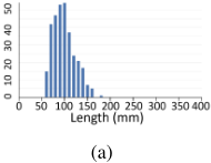
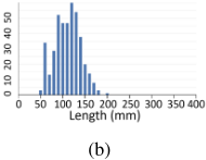
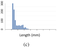
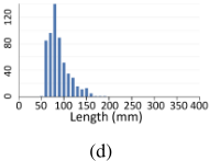
A deeper understanding of fish population dynamics facilitates effective decision making in dynamic habitats.
Modeling growth and survival is challenging for several reasons. First, we need to consider impacts of multiple environmental drivers that can jointly influence population dynamics through complex pathways [Ozgul et al., 2009; Coulson et al., 2011; Pelletier et al., 2012]. Second, there is often strong variability in fish patterns through space (e.g., across different rivers) and over time (e.g., across seasons and fish cohorts). Fig. 1 shows the seasonal distribution of body length values for all the brook trout (Salvelinus fontinalis) captured around the West Brook watershed in western Massachusetts. This shows the variability of fish body size due to the change of season and weather conditions. Third, the collected individual fish data are often sparse as probabilities of capture are almost always less than 1 and generally much lower [Letcher et al., 2015] and fish can emigrate from study areas [Letcher et al., 2005]. The available data can also be biased towards certain locations, seasons, or fish cohorts. Moreover, the growth data (e.g., fish length) can be noisy (+/- 1 mm) due to measurement errors in the field and the variability in growth among individuals.
Aquatic ecologists often build Bayesian models to study fish survival and body growth. For example, Letcher et al. [Letcher et al., 2015] built a Bayesian framework with latent state variables to estimate the effects of environmental variation on interactive components of fish population dynamics. The model consists of modules for modeling fish survival, body growth, movement among rivers, and individual capture probability. These Bayesian models are widely used because they can explicitly represent the internal relationships amongst different variables, implicitly account for uncertainty in parameter estimates and can effectively propagate the uncertainty through multiple interacting states [Raabe et al., 2014; Kanno et al., 2015; Letcher et al., 2015]. However, efficacy of Bayesian models for large, complex datasets can be limited. First, traditional Bayesian approaches commonly use Gibbs sampling for parameter estimation, which can result in very long and impractical run times (i.e., weeks) for modeling complex data, e.g., a large number of individual fish [Belloni and Chernozhukov, 2009]. Second, Bayesian models reach an upper practical limit in model complexity as additional drivers and interactions are incorporated [Heckerman, 1998]. As an alternative, machine learning models have also been developed for modeling species population dynamics [Seo et al., 2021; Joseph, 2020; Mohankumar and Hefley, 2022; Bonnaff´e et al., 2021], but they ignore underlying processes and complexity used in Bayesian models and also consider target variables independently without modeling their dependencies, e.g., the relation between survival and variables such as body length and weight. Moreover, both existing machine learning and Bayesian models can be affected by data availability and bias across space and time [Xie et al., 2021a; Xie et al., 2021b]. As a result, model performance can be variable across locations and cohorts. Bayesian models account for variable data availability by using hierarchical model structures where information is shared across sites and time, but so far none of the existing methods have considered uneven data variability across cohorts.
In this paper, we propose a new neural network model, Coupled Growth-Survival network (CGS), for modeling fish body growth and survival. The CGS model explicitly captures the dependencies between the dynamics of fish survival, fish capture probability, and environmental variations in a Bayesian structure. It also takes into account the effect of body size on fish survival by coupling a separate growth model and the survival model. The growth model predicts the fish growth rate in each season and uses the observed fish length as labels in the training process. It also enforces the prior knowledge about fish growth patterns into the learning process. Additionally, we propose two learning strategies to mitigate the performance disparity across cohorts. First, an adaptive model refinement method is developed to adjust training priorities for different fish cohorts based on their predictive performance. Second, we create a data augmentation method to address the data sparsity and imbalance issues. Specifically, we create pseudo labels through an individual re-calibration process. Then we estimate the confidence for these pseudo labels using a Bayesian model as a teacher.
Then we re-train the growth model by incorporating pseudo labels while using their confidence as sample weights.
We evaluate the proposed method using real-world data collected from a stream network located in western Massachusetts, US. The results demonstrate the effectiveness of the proposed method in improving the prediction of fish growth and survival and also preserving the fairness across different fish cohorts. The fish growth and movement patterns discovered by the proposed model are also consistent with prior studies in the same region [Letcher et al., 2015]. Moreover, compared to traditional Bayesian-based fish models, the proposed method can significantly reduce run times (weeks to ∼30mins) and memory requirements (10's gB of RAM vs ∼5gB).
2 ProblemDefinition
In this problem, we consider N fish samples from M rivers. We use r as the index of rivers, and use i as the index for fish samples. For each individual fish i, we use the input features xti at each time t, which include variables describing the environmental conditions, such as water flow and water temperature, as well as the information of season, cohort, and current river id.
We consider every season as a time step. For every time step t, our objective is to (1) model whether each fish survives (i.e., ztir = 1) at a specific river site r, and (2) predict the body length ˆ yt i for each fish. In the training process, we use the fish observation (survival) data O and body length data Y from [Letcher et al., 2015]. In particular, O = {otir }, where otir = 1 indicates that the fish i is observed in river r at time t. Fish length data are represented as Y = {yt i }, where yt i is the measured body length (in mm) for fish i at time t. It is noteworthy that both the observation and body length data are sparse as fish may not be captured at each time step even while they are still alive.
We also aim to promote the fairness of a learning model's performance on the body length prediction over several mutually-exclusive groups of individual fish. Here we consider the fairness objective as reducing the performance disparity across different fish groups. For example, the fairness metric can be the standard deviation of root mean squared error (RMSE) over all the groups. In this work, groups are defined by fish cohorts. The fairness aims to ensure the balance of model performance across all fish cohorts.
3 Method
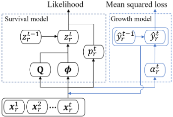
The overall flow of the proposed method is shown in Fig. 2. The fish survival Ms depends not only on input features (e.g., environmental conditions, seasons, cohorts), but also on their current body size [Letcher et al., 2015]. We create a fish growth modeling component Ml for predicting the body length of each fish. The output of Ml is fed to the survival model Ms as an additional input. The entire model is trained in an end-to-end fashion so the two components Ms and Ml can supplement each other. In this section, we first describe the survival modeling component Ms and the body length modeling component Ml. Then we introduce new fairness enforcement methods to reduce the performance disparity over different fish cohorts.
3.1 Survival Model
We first introduce an independent survival model without considering the effect of fish body size. Inspired by prior work [Royle, 2008; Letcher et al., 2015], we consider the fish survival as a Markov process, in which the survival at time t depends on the previous survival state at t - 1. In particular, we use the survival indicator ztir = 1 to represent that the fish i is alive and stays in river r at time t. The survival of a fish in river r at the next time step t + 1 depends on (1) whether the fish is alive at t, (2) the probability for the fish to move to river r before time t+1, and (3) the probability for the fish to survive from t to t + 1. To capture such relationships, we introduce a variable ϕtir to represent the probability for the fish i to keep surviving in river r at time t + 1, i.e., ϕtir = P(zt+1 ir = 1|zt→ ir = 1), where zt→ ir = 1 indicates that the fish stays or arrives at river r at a time during [t,t + 1).
The variable ϕtir is sampled from a Gaussian distribution ϕtir ∼ N(µtϕ,ir , σtϕ,ir ), where the mean and standard deviation are computed from the input features through functions specific to river r, as follows:
where the functions f r 1 and f r 2 are river r-specific functions and are implemented using multi-layer neural networks. we adopt the reparameterization trick [Kingma and Welling, 2013] to ensure the differentiability of the sampling process of ϕtir .
We then create a transition matrix Qti for the time window [t, t + 1), where Qti (r, r′ ) denotes the probability for the fish i to move from river r to river r′ during the time window [t,t + 1]. Each row r of the transition matrix Q is computed as:
where the function qr is specific to river r and implemented by a multi-layer network with a softmax output.
Then we sample the survival variable ztir at time t from a Bernoulli distribution. The parameter of the Bernoulli distribution needs to consider the survival of the fish i at the previous time t-1, the movement to the river r, and the probability for it to keep surviving. This process is expressed as follows:
Ideally, we wish to compare the modeled survival variables z with fish observations O. However, for each fish, it may not be captured every time even when it survives. Hence, we create another capture probability variable pti = d(xti ), where d is a multi-layer network with a sigmoid output in [0,1].
Combining the survival variables, the capture probability, and observations, we define the training objective using the negative log-likelihood function, as follows:
The model parameters in functions f1, f2, q, and d are updated by minimizing the loss function via back-propagation. It is noteworthy that the sampling process by Eq. 3 is not differentiable. There are two possible solutions to overcome this issue: (1) using the Gumbel-softmax reparamererization for the Bernoulli sampling [Jang et al., 2016], and (2) directly using the Bernoulli probability P(ztir = 1) as the value of ztir in Eq. 4 without sampling. We notice that the second approach yields slightly better performance in our tests.
3.2 Fish GrowthModeling
We build a predictive model g to predict the fish growth at each time step. According to prior studies [Sigourney et al., 2008; Letcher et al., 2015], environmental conditions can affect how fast the fish grow over time. Hence, instead of directly predicting the body length value yt i at t, the model g is designed to predict the length increase (i.e., growth rate) for each fish from each time t to the next step t + 1. Specifically, we represent the growth rate of fish length as
where x:t i represents the input features for the fish i until the time step t. The function g is implemented by a Long-Short TermMemory (LSTM) model [Hochreiter and Schmidhuber, 1997] and a softplus output layer, which ensures the growth value αt i is non-negative. The noise term ei ∼ N(µi, σi) accounts for the fish individual difference and the observation errors, and is constant over time.
After we obtain the predicted growth rates, we estimate the length of fish at each time t as
where y1 i is the body length of fish i at the first time step (first obervation for each fish). Here we assume that all the fish samples in our study have observed initial body length values. The growth model is trained by minimizing the mean-squared error (MSE) by comparing with observed fish length values.
Besides the effect of environmental conditions, the growth rate also depends on the current fish body size [Hopkins, 1992]. Hence, we build a recurrent process by feeding the predicted length values ˆ yt-1 i (Eq. 6) at the previous time as additional input to predict the growth rate at time t. Then Eq. 7 is updated asαt i = g([x:t i , ˆ yt-1 i ]) + ei, (7)
Coupled growth-survival model: Prior study has demonstrated the interplay between fish survival and body size [Letcher et al., 2015; Lorenzen et al., 2022]. Hence, we enhance the survival modeling by augmenting the input variable ˜xtir = [xtir , ˆ yt i ], which is then fed to the functions f1, f2, q and d. The growth model and the survival model are jointly trained in an end-to-end fashion so the survival uncertainty will be propagated to update the growth model.
Incorporating knowledge constraints: The observed body length values are sparse for many fish samples. Training the growth model using such sparse data can lead to the degradation of the accuracy and also the inconsistency with known growth patterns. In particular, we notice that the model g(·) learned using sparse data produces smooth growth rates over different seasons. According to prior fish studies [Sigourney et al., 2008; Letcher et al., 2015], fish often grow much faster from spring to summer compared to other seasons. To account for this issue, we propose to enforce the prior knowledge about fish growth patterns into the learning process. To capture such variation, we introduce a bias term bti = u(xti ), where u is a transformation function implemented by fullyconnected neural networks. Then the growth rate can computed as
3.3 Fairness Enforcement
The fish cohort-related biases can be caused by both the unfair learning process and the sparse training samples. These biases are especially hurtful for monitoring the growth and survival of fish populations. Amongst existing fairnessenforcing methods, the most common strategy is to incorporate additional fairness losses as the term in the loss function [Zafar et al., 2017; Yan and Howe, 2019; Kamishima et al., 2011; Serna et al., 2022], e.g., L = Lpred + λ · Lfair, where Lpred is the prediction loss (e.g., MSE loss) and λ is a scaling factor. Another major direction involves incorporating additional discriminators during training to penalize learned representations that may reveal the identity of a group (e.g., gender) in an adversarial manner. [Sweeney and Najafian, 2020; Zhang and Davidson, 2021; Alasadi et al., 2019]. However, these fairness-preserving methods face three main limitations when used for fish cohort fairness: (1) In deep learning training, mini-batches are often used due to data size, but it is difficult for each mini-batch to contain representative samples from all cohorts when calculating Lfair. (2) The choice of scaling factor λ directly impacts the final output and varies from problem to problem. If not properly set, the scaling factor may lead to direct competition between Lpred and Lfair. (3) Existing methods can still be affected by sparse and imbalanced training samples.
To mitigate these concerns, we introduce two approaches for enforcing fairness. The first approach, adaptive model refinement, aims to adjust the priority of training over different fish cohorts. The second approach, data augmentation with uncertainty, aims to enhance the model training with additional pseudo-labels.
Adaptive model refinement: The standard predictive model g may comprise the performance on certain cohorts to achieve better overall performance. To address this issue, we introduce a global referee to evaluate the performance disparity during the training process and identify the cohorts that are under-represented by the current predictive model g, as inspired by the previous work [Xie et al., 2022; He et al., 2022]. Then the referee will adjust the learning rate for different cohorts based on their relative performance. The advantage of this method is in that it disentangles the fairness objective and the performance optimization.
Specifically, in each iteration, the referee evaluates the performance (e.g., RMSE) Mc on each fish cohort c ∈ C, and measures its deviation with the overall performance ¯M. In our tests, we measure the overall performance ¯M as the RMSE of the current model g over all the observation data. We then modify the learning rate ηc for the cohort c as
where ηinit is the learning rate used to train model g, η′min = argminη′c {η′c | η′c , ∀c ∈ C}, and η′max = argmaxη′c {η′c | ∀c ∈ C}.
According to Eq. 9, if a cohort's performance Mc is worse than the overall performance, its learning rate ηc will be increased relatively to other cohorts. As a result, the samples in this cohort will have a higher impact for training the predictive model g. Moreover, all the learning rates after the update are normalized back to the range [0, ηinit] to keep the optimization process stable.
Data augmentation with uncertainty. The performance disparity can be exacerbated by the lack of represensative training samples. To address this issue, we propose to impute missing observations and then use the imputed data with a reweighting strategy to augment the training process.
In particular, for each fish, we first apply the obtained model g to predict body length values over all the time steps using the current model. Then we refine the predicted values through an individual re-calibration process. The intuition is that, for any fish with at least two body length observations, the predicted growth rates need to be consistent with the increase of body length values. Specifically, we propose to update the noise factor ei in Eq. 8 separately for each pair of consecutive observed length values, e.g., between time t1 and t2, and then apply the obtained noise factor to each time step from t1 to t2-1 in the prediction. If the observation at t2 is the last observation, we will keep using the obtained noise factor until the end of the observation period.
Next, we will use the re-calibrated values ˜αt i as pseudolabels for training the model by including another MSE loss Laug between the predicted growth rates αt i and the recalibrated values ˜αt i . Since the re-calibrated growth rates are not fully accurate, we reweight them based on the uncertainty of a separate Bayesian model. In particular, we follow the prior work [Letcher et al., 2015] to create a linear probabilistic growth model, with the input of water flow, water temperature, the product of water flow and water temperature, and the body length. Then we use this model to estimate P(˜αt i |xti ). The obtained probability density values are normalized over all the samples and used to reweight the re-calibrated growth rates in the MSE loss Laug.
4 Experiments
4.1 Dataset
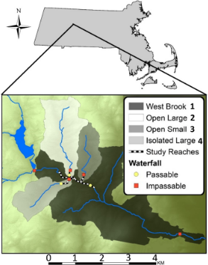
The fish data are collected from the West Brook (WB) and three tributaries, located in western Massachusetts, US (Fig. 3). The focal study area consists of a 1-km long reach of the WB and 300-m long reaches of three tributaries (rivers 2-4). The bottom of the study area on river 4 contains a waterfall, which blocks access to river 4 from the WB (river 1). Average stream width is 4-5 m for the WB, and 1-3 m for tributaries. Fish were captured using standard stream ecology techniques (details in [Letcher et al., 2015]) in the four rivers four times per year (seasonally) from 2002 to 2015. Upon capture, fish were anesthetized, measured for length (+/- 1 mm) and a 12-mm Passive Integrated Transponder tag was inserted through a small incision in the abdomen. The tag provided a unique ID for each tagged fish.
In this work, we focus on modeling the survival and growth of brook trout (Salvelinus fontinalis) in the study region. We study in total 11,768 fish samples from 13 cohorts. Each cohort is defined as the set of fish of the same age. We model the survival and body length for each fish over a 3 year period by treating each season as a time step. The survival and length observations are only available for certain time steps (when a fish was captured). In total we have 23,760 survival observations over 4 river sites and 23,748 length observations.
4.2 Accuracy Evaluation
We first evaluate the accuracy of the proposed methods in modeling fish growth and survival. In particular, we compare the predicted body length and survival values with observations. We evaluate the model performance by splitting all the fish samples into disjoint training and testing set. We also adjust the ratio of samples in the training set, i.e., using 1%, 10%, and 50% of all the fish samples for training, and test the obtained model in the remaining fish samples.
We implemented the proposed method using computer technology for high performance [Window 11, CPU i9 13900F, GeForce RTX 3080 GPU]. The intermediate transformation functions (e.g., f1, f2, q, d, u) are implemented as a two-layer network with the intermediate layer of 20 hidden units using the sigmoid activation function. The function g is implemented using a standard one-layer LongShort Term Memory (LSTM) [Hochreiter and Schmidhuber, 1997] with the hidden representation of 10 dimensions.
The initial learning rate ηinit for the training is set as 0.01. Code is available at: https://drive.google.com/drive/folders/ 1dPtJ1eU-u YQwKaRAtNScUonfeW0fEbZ.
Body length prediction: Table 1 summarizes the performance of multiple different methods in predicting body length using different numbers of training fish samples (1%, 10%, 50%). In particular, the Recurrent Neural Networks (RNN) model is a standard RNN neural network with the LSTM cell [Hochreiter and Schmidhuber, 1997], and it takes the input x and outputs the growth rates. The RNNauto extends the RNN model with another autoregressive structure by feeding the predicted body length value as input to the next time step. The CGS model is the proposed model in which the growth model is coupled with the survival model. CGSfair enforces the fairness on the CGS model using the adaptive model refinement approach. CGSfair-ps further uses the pseudo-labels to augment the training process (Section 3.3). The performance is measured in terms of the overall RMSE (i.e., measured over all the observed length values) and the sample-wise RMSE (i.e., measured over each fish separately and then averaged over all the fish samples).
It can be seen from Table 1 that the proposed CGS model outperforms the independent growth models (i.e., RNN and RNNauto), which shows the benefit of training survival and growth models together. The improvement from RNN to RNNauto confirms the benefit of including the previous predicted length values as input. This improvement is less obvious when the model is trained using less training data because the predicted length values are less accurate. The adaptive model refinement method can slightly improve the predictive accuracy as it dynamically increases the training priority over under-represented cohorts. The use of pseudo-labels can improve the performance as it better exploits the individual difference through the individual re-calibration process and augment the sparse training data with additional supervision.
Fig. 4 shows examples of predicted body length values by different methods. Fig. 4 (a)-(c) shows the results for the same fish but using different amounts of training data (1%, 10%, 50%), and Fig. 4 (d) shows the result for a different fish using 10% training data. We observe that the standard RNN method can over-estimate or under-estimate the length values when using less training data, and the accumulated error becomes larger over time. When using more training samples, all the methods have much better performance.

| Method | 1% | 10% | 50% |
|---|---|---|---|
| RNN | 12.44(8.31) | 9.15(7.12) | 7.96(5.43) |
| RNNauto | 12.29(8.22) | 8.39(5.98) | 7.47(5.21) |
| CGS | 11.39(7.33) | 7.88(5.65) | 7.26(5.13) |
| CGSfair | 11.19(7.19) | 7.64(5.34) | 7.21(5.12) |
| CGSfair-ps | 11.10(7.19) | 7.60(5.31) | 6.87(4.99) |
| Method | 1% | 10% | 50% |
|---|---|---|---|
| Independent | 0.87 (0.81) | 0.87 (0.81) | 0.87 (0.82) |
| CGS | 0.89 (0.84) | 0.89 (0.85) | 0.90 (0.85) |
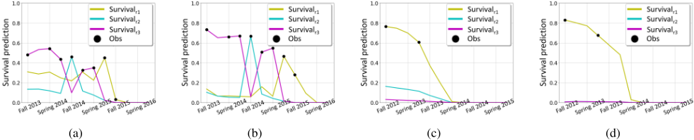
Survival modeling: We also test the effect of integrating the body length modeling into the survival modeling component. The comparison is shown in Table 2. Here we report the average likelihood of all the observed survival data and the average likelihood of the survival data when fish move across different river sites. Modeling survival with movement is more challenging as the model needs to correctly predict both the target river site and the survival value. According to the results, we can observe that the coupled model can achieve better performance in modeling fish survival. Fig. 5 shows the survival indicators predicted by the independent and coupled models in two fish samples. The results in Fig. 5 (a) and (c) are produced by the independent survival model, while the results in Fig. 5 (b) and (d) are generated by the CGS model. For the first sample (Fig. 5 (a) and (b)), we can see that the coupled model can better capture the movement of fish across different river sites, especially when the fish enters river 3 the second time. For the second sample (Fig. 5 (c) and (d)), the fish stays in the same river (river 1) all the time. The coupled model is shown to produce higher survival values on the river 1 while the independent model still outputs survival values for other rivers.
| Method | 1% | 10% | 50% |
|---|---|---|---|
| CGS | 2.37(3.53) | 1.78(2.62) | 1.25 (2.43) |
| CGSfair | 2.14(2.90) | 1.49(1.94) | 0.93(1.63) |
| CGSfair-ps | 2.11(2.93) | 1.47(1.92) | 0.86(1.58) |
4.3 Fairness Evaluation
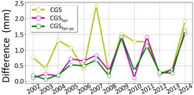
Table 3 shows the performance disparity across cohorts in predicting body length by three methods. We include two sets of measures: (1) the standard deviation of RMSE over all the cohorts; and (2) the maximum distance between the RMSE of a cohort and the overall RMSE. As we can see, the CGSfair method greatly reduces the disparity across cohorts by using the adaptive refinement approach. And the incorporation of pseudo-labels (CGSfair-ps) further promotes the performance fairness. Fig. 6 shows the absolute difference between the RMSE of each cohort and the overall RMSE using 50% training data. For the CGS model, the lack of consideration on fairness leads to larger errors for some cohorts (i.e., cohort 2007). This is because prediction accuracy for one cohort can be easily compromised to pursue better results for other cohorts, which can cause the performance degradation for certain cohorts. In contrast, the proposed fairness enforcement methods can effectively reduce the absolute difference for most cohorts.
4.4 Growth andMovement Analysis
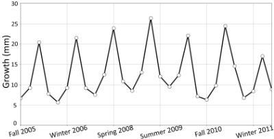
We aim to analyze the fish growth and movement patterns using the obtained CGS model. Fig. 7 shows the growth rates of body length at each time step (season). It can be seen that the fish grows much faster in Spring season (i.e., from Spring to Summer), likely due to increasing temperatures and high prey availability [Grade and Letcher, 2006], This is also consistent with the previous fish modeling study for the same data [Letcher et al., 2015].
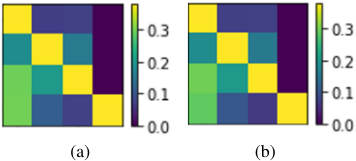
We also plot the movement matrices across four rivers in Fig. 8. It can be seen that most fish tend to stay in the same river. The light region in the first column shows that a certain number of fish move from their original rivers to the river 1, which is the main stream connecting to rivers 2-4. The model also predicts that no fish move to river 4, which is justified by the fact that there is a waterfall at the entrance of river 4.
5 Conclusion
In this work, we propose a new model for predicting fish survival and body growth in multiple connected rivers. The proposed method (CGS) models fish survival as a Markov process and integrates the effect of environmental variables in a neural network. It also couples the modeling of survival and growth so the two components can inform each other. Two fairness enforcement approaches are also developed to reduce the performance disparity over different fish cohorts. We have several observations from our experiments in a realworld fish dataset: (1) The CGS method can achieve superior performance than independent models in modeling survival and body lengths. (2) The CGS method can achieve reasonable performance even using a small number of training samples. (3) The proposed adaptive refinement method and the data augmentation can help the model preserve the fairness across cohorts while also slightly improving the performance. (4) The fish growth and movement patterns discovered by the CGS model are consistent with previous studies in the same region, while vastly reducing run times (weeks to ∼30mins) and memory requirements (10's gB of RAM vs ∼5gB).
The proposed method remains limited in modeling multiple fish species, e.g., Atlantic salmon (Salmo salar) and brown trout (Salmo trutta) in the same study area. In the future, one could explore differences in growth and survival and interactions amongst the species. One could also potentially explore growth and survival variation at finer spatial scales (10's of m vs the current scale of 1 km). The proposed method is also applicable to studying many other animal species with complex data in complex ecosystems.
Acknowledgments
This work was supported by the USGS awards G22AC00266 and G21AC10564, the NSF awards 2147195, 2105133, and 2126474, the NASA award 80NSSC22K1164, Google's AI for Social Good Impact Scholars program, the Pitt Momentum Award, and the DRI award at the University of Maryland. Any use of trade, firm, or product names is for descriptive purposes only and does not imply endorsement by the U.S. Government. Animal care and use protocols are identified in Eastern Ecological Science Center study plan 71-LB00TGF.
@inproceedings{ijcai2023p664,
  title     = {CGS: Coupled Growth and Survival Model with Cohort Fairness},
  author    = {He, Erhu and Wan, Yue and Letcher, Benjamin H. and Fair, Jennifer H. and Xie, Yiqun and Jia, Xiaowei},
  booktitle = {Proceedings of the Thirty-Second International Joint Conference on
               Artificial Intelligence, {IJCAI-23}},
  publisher = {International Joint Conferences on Artificial Intelligence Organization},
  editor    = {Edith Elkind},
  pages     = {5986--5994},
  year      = {2023},
  month     = {8},
  note      = {AI for Good},
  doi       = {10.24963/ijcai.2023/664},
  url       = {https://doi.org/10.24963/ijcai.2023/664},
}
TY - CPAPER TI - CGS: Coupled Growth and Survival Model with Cohort Fairness AU - He, Erhu AU - Wan, Yue AU - Letcher, Benjamin H. AU - Fair, Jennifer H. AU - Xie, Yiqun AU - Jia, Xiaowei T2 - Proceedings of the Thirty-Second International Joint Conference on Artificial Intelligence, IJCAI-23 PB - International Joint Conferences on Artificial Intelligence Organization PY - 2023 SP - 5986 EP - 5994 DO - 10.24963/ijcai.2023/664 UR - https://doi.org/10.24963/ijcai.2023/664 ER -Copied
Machine-readable versions of this paper, for tools and AI agents:





