
Optimization-driven Demand Prediction Framework for Suburban Dynamic Demand-Responsive Transport Systems
Proceedings of the Thirty-Second International Joint Conference on Artificial Intelligence. AI for Good. Pages 6335-6342.
https://doi.org/10.24963/ijcai.2023/703
Keywords
- AI for Good: Machine Learning
- AI for Good: Constraint Satisfaction and Optimization
- AI for Good: Planning and Scheduling
Abstract
Demand-Responsive Transport (DRT) has grown over the last decade as an ecological solution to both metropolitan and suburban areas. It provides a more efficient public transport service in metropolitan areas and satisfies the mobility needs in sparse and heterogeneous suburban areas. Traditionally, DRT operators build the plannings of their drivers by relying on myopic insertion heuristics that do not take into account the dynamic nature of such a service. We thus investigate in this work the potential of a Demand Prediction Framework used specifically to build more flexible routes within a Dynamic Dial-a-Ride Problem (DaRP) solver. We show how to obtain a Machine Learning forecasting model that is explicitly designed for optimization purposes. The prediction task is further complicated by the fact that the historical dataset is significantly sparse. We finally show how the predicted travel requests can be integrated within an optimization scheme in order to compute better plannings at the start of the day. Numerical results support the fact that, despite the data sparsity challenge as well as the optimization-driven constraints that result from the DaRP model, such a look-ahead approach can improve up to 3.5% the average insertion rate of an actual DRT service.
- [Agency, 2023] International Energy Agency. Global co2 emissions from transport by subsector, 2000-2030. https://www.iea.org/data-and-statistics/charts/global-co2- emissions-from-transport-by-subsector-2000-2030, 2023. Accessed: 2023-02-23. Link
- [Bernardo and Pannek, 2018] Marcella Bernardo and Jürgen Pannek. Robust solution approach for the dynamic and stochastic vehicle routing problem. Journal of Advanced Transportation, 2018, 2018.
- [Codato and Fischetti, 2006] Gianni Codato and Matteo Fischetti. Combinatorial benders' cuts for mixed-integer linear programming. Operations Research, 54(4):756- 766, 2006.
- [Cordeau and Laporte, 2007] Jean-Franc ¸ois Cordeau and Gilbert Laporte. The dial-a-ride problem: models and algorithms. Annals of operations research, 153(1):29, 2007.
- [Fachini and Armentano, 2020] Ramon Faganello Fachini and Vinícius Amaral Armentano. Logic-based benders decomposition for the heterogeneous fixed fleet vehicle routing problem with time windows. Computers & Industrial Engineering, 148:106641, 2020.
- [Feigon and Murphy, 2016] Sharon Feigon and Colin Murphy. Shared mobility and the transformation of public transit. Transportation Research Board, 2016.
- [Ferreira et al., 2013] Nivan Ferreira, Jorge Poco, Huy T Vo, Juliana Freire, and Cláudio T Silva. Visual exploration of big spatio-temporal urban data: A study of new york city taxi trips. IEEE transactions on visualization and computer graphics, 19(12):2149-2158, 2013.
- [Ho et al., 2018] Sin C Ho, Wai Yuen Szeto, Yong- Hong Kuo, Janny MY Leung, Matthew Petering, and Terence WH Tou. A survey of dial-a-ride problems: Literature review and recent developments. Transportation Research Part B: Methodological, 111:395-421, 2018.
- [Hochreiter and Schmidhuber, 1997] Sepp Hochreiter and Jürgen Schmidhuber. Long short-term memory. Neural computation, 9(8):1735-1780, 1997.
- [Johnson, 1967] Stephen C Johnson. Hierarchical clustering schemes. Psychometrika, 32(3):241-254, 1967.
- [Liu et al., 2019] Lingbo Liu, Zhilin Qiu, Guanbin Li, Qing Wang, Wanli Ouyang, and Liang Lin. Contextualized spatial-temporal network for taxi origin-destination demand prediction. IEEE Transactions on Intelligent Transportation Systems, 20(10):3875-3887, 2019.
- [Riedler and Raidl, 2018] Martin Riedler and Günther Raidl. Solving a selective dial-a-ride problem with logic- based benders decomposition. Computers & Operations Research, 96:30-54, 2018.
- [Saint-Guillain et al., 2015] Michael Saint-Guillain, Yves Deville, and Christine Solnon. A multistage stochastic programming approach to the dynamic and stochastic vrptw. In Integration of AI and OR Techniques in Constraint Programming: 12th International Conference, CPAIOR 2015, Barcelona, Spain, May 18-22, 2015, Proceedings 12, pages 357-374. Springer, 2015.
- [Tensen, 2015] IF Tensen. Stochastic optimization of the dial-a-ride problem. dealing with variable travel times and irregular arrival of requests in the planning of special transport services. Master's thesis, University of Twente, 2015.
- [Tong et al., 2017] Yongxin Tong, Yuqiang Chen, Zimu Zhou, Lei Chen, Jie Wang, Qiang Yang, Jieping Ye, and Weifeng Lv. The simpler the better: a unified approach to predicting original taxi demands based on large-scale online platforms. In Proceedings of the 23rd ACM SIGKDD international conference on knowledge discovery and data mining, pages 1653-1662, 2017.
- [Toqué et al., 2016] Florian Toqué, Etienne Côme, Mohamed Khalil El Mahrsi, and Latifa Oukhellou. Forecasting dynamic public transport origin-destination matrices with long-short term memory recurrent neural networks. In 2016 IEEE 19th international conference on intelligent transportation systems (ITSC), pages 1071-1076. IEEE, 2016.
- [Vallée, 2019] Sven Vallée. Algorithmes d'optimisation pour un service de transport partagé à la demande. PhD thesis, Université de Lorraine, 2019.
- [Wang et al., 2019] Yuandong Wang, Hongzhi Yin, Hongxu Chen, Tianyu Wo, Jie Xu, and Kai Zheng. Origin- destination matrix prediction via graph convolution: a new perspective of passenger demand modeling. In Proceedings of the 25th ACM SIGKDD international conference on knowledge discovery & data mining, pages 1227-1235, 2019.
- [Yang et al., 2017] Chao Yang, Fenfan Yan, and Xiangdong Xu. Daily metro origin-destination pattern recognition using dimensionality reduction and clustering methods. In 2017 IEEE 20th International Conference on Intelligent Transportation Systems (ITSC), pages 548-553. IEEE, 2017.
- [Yao et al., 2018] Huaxiu Yao, Fei Wu, Jintao Ke, Xianfeng Tang, Yitian Jia, Siyu Lu, Pinghua Gong, Jieping Ye, and Zhenhui Li. Deep multi-view spatial-temporal network for taxi demand prediction. In Proceedings of the AAAI conference on artificial intelligence, volume 32, 2018.
- [Zhuang et al., 2022] Dingyi Zhuang, Shenhao Wang, Haris Koutsopoulos, and Jinhua Zhao. Uncertainty quantification of sparse travel demand prediction with spatial-temporal graph neural networks. In Proceedings of the 28th ACM SIGKDD Conference on Knowledge Discovery and Data Mining, pages 4639-4647, 2022.
- [Zigrand et al., 2021] Louis Zigrand, Pegah Alizadeh, Emiliano Traversi, and Roberto Wolfler Calvo. Machine learning guided optimization for demand responsive transport systems. In Machine Learning and Knowledge Discovery in Databases. Applied Data Science Track: European Conference, ECML PKDD 2021, Bilbao, Spain, September 13-17, 2021, Proceedings, Part IV 21, pages 420-436. Springer, 2021.
References were extracted automatically from the PDF and may contain errors.
Full text extracted automatically from the PDF; figures, tables and equations may differ. The PDF is the version of record.
1 Introduction
Individual cars, buses and taxis were held responsible for around 45% of the CO2 emitted around the world by the transportation sector in 2020, which accounts for 24% of all CO2 emissions globally [Agency, 2023]. One solution to tackle this environmental issue is to have a better use of the existing transportation resources through shared mobility systems. In particular, Demand-Responsive Transport defines shared transport systems where the vehicles adapt their routes dynamically to the demand rather than using fixed routes and timetables. It aims at improving public transportation in areas with a low population density such as the suburbs of large cities [Feigon and Murphy, 2016].
This work has been performed in collaboration with Padam Mobility, an international company that has developed software solutions to efficiently manage Demand-Responsive Transport services for almost a decade in partnership with local and regional public transport authorities. Such a long lasting collaboration allows us to leverage a large volume of data to define a proper Big Data analysis project with regards to the mobility needs in some of their oldest territories.
2 Overview
We explain in this work how we can take advantage of some historical records to enable Demand-Responsive Transport services to be more flexible and thus more available.
In short, travel requests can be performed days in advance as well as just a few minutes before the requested departure time. We are interested in building an initial planning for the drivers at the start of the operational day that takes into account predicted requests that could happen during the day.
We first present some statistics using the available data and we show how the pre-processing can manage the sparsity and the heterogeneity of the demand, the two main challenges related to the forecasting task on the considered territories. We then discuss how the Dial-a-Ride Problem, that is the optimization model used in Demand-Responsive Transport, is affected by the obtained prediction. In light of that relation, we investigate how the available data should be pre-processed to have the most beneficial impact on the optimization model. We present the performances of a Moving Average and a LSTM models used as Demand Prediction Frameworks that are precisely tailored for obtaining an optimization model able to provide high-quality solutions. Finally, we prove the overall effectiveness of the proposed framework by plugging this prediction into the Offline Optimization Process and by performing simulations that pinpoint the margin for improvement with respect to the myopic insertion algorithms currently used in practice.
The major contributions of this work are the following:
- We depict the particularities of Demand-Responsive Transport services in suburban areas through a detailed numerical study of the available data;
- We explain how a Demand Prediction Framework can be used in tandem with a Dynamic Dial-a-Ride
Problem solver and how this interaction drastically affects the requirement on the prediction model itself;
- We pinpoint the difficulties met when modeling such a Machine Learning model in terms of performance;
- We present numerical insights based on simulations into the potential of developing a Demand Prediction tool for Demand-Responsive Transport systems.
3 Data Analysis
In the transportation field, most of the works that can be found in the literature around "Origin-Destination-TimeSlot" prediction revolve around large scale service offers, such as taxis [Liu et al., 2019], subways [Yang et al., 2017] or public transport services [Toqu´e et al., 2016] in big cities. Most of the closely-related works focus on "Origin-TimeSlot" prediction only [Tong et al., 2017; Yao et al., 2018]. Those datasets have the advantage of being open access and massive in terms of volume: for instance, New-York yellow taxis account for hundreds of millions of historical travel requests over the years [Ferreira et al., 2013]. Such quantities allow Deep Learning techniques to be considered to forecast future mobility needs. Additionally, those papers mostly target short-term predictions with a rolling horizon of 15 to 60 minutes and can consider wide departure and destination zones up to a few km2 [Wang et al., 2019].
Our work is focused on suburban areas where mobility needs are way more heterogeneous and sparse. Hence, instead of having more than a hundred million travel requests performed each year in a rather small and dense area, we consider only up to a few hundred thousands travel requests performed each year in a really wide area. We also focus on "Origin-Destination-TimeSlot" prediction because we want to obtain an estimation of the demand for the whole next operational day to optimize the initial plannings.
To understand the specificities and complexities of rural and suburban mobility needs through a detailed numerical analysis, we first introduce a few concepts.
We note N = {Ni = (lati, lngi )}i∈[[1,nbus stops]] the set of bus stops where travelers can be served, defined by their latitude and longitude coordinates. The set N defines the geography of the considered transportation offer. We then note R as the set of historical travel requests for this Demand-Responsive Transport service. For each r ∈ R, we know (lat departure r , lng departure r ) the coordinates of the departure location, (lat destination r , lng destination r ) the coordinates of the destination location, and time departure r the requested time of pick-up at the associated departure bus stop.
The N and R sets constitute the raw data that we have.
Regarding the raw data, most of the travel requests are unique if we only look at the bus stop of departure, the bus stop of arrival and the requested departure time. Consequently, in order to bring out patterns in the mobility needs from our dataset, we decide to group the travel requests into clusters of similar demand so that they do not all look like distinct and exceptional events.
We thus define the concept of "Aggregated Travel Requests" based on a geographical threshold ∆D in meters and a temporal threshold ∆T in minutes. Aggregations are performed sequentially, geographically first and temporally second. As shown in Figure 1, we want to cluster the historical travel requests into travel requests from a departure zone to a destination zone with a departure time slot in the day. In this example, R1 and R2 are grouped together in ({N1,N2} , {N3,N4,N5} , [10:00, 10:15]) while R3 is put in ({N1,N2} , {N3,N4,N5} , [10:20, 10:25]).
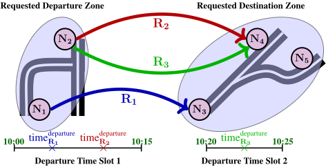
To achieve this objective, we first compute a clustering Z of the bus stops such that the diameter of each cluster is below the ∆D threshold, as described in Equation (1). For this clustering phase, distance G is the Haversine formula.
This particular aggregation of bus stops can be heuristically obtained using Hierarchical Clustering [Johnson, 1967].
Based on this geographical clustering, we can assign each historical travel request r ∈ R to a departure Z r departure and a destination Z r destination zones as detailed in Equations (2-3).
Based on those definitions, we can aggregate a first time the historical travel requests based on their departure and destination zones, as written in Equation (4).
We can then aggregate those spatially clustered travel requests per similar requested times of pick-up as described in Equation (5). For each (Z1,Z2) ∈ Z 2 , we search time slots of departure smaller than ∆T to obtain ATZ1,Z2 , a set of clusters of travel requests from Z1 to Z2 with close enough requested departure times, such as [10:00, 10:15]. Here, distance T is the difference in minutes between two daily timings. For instance, distance T (23:42, 00:07) = 25.
Those definitions allow us to properly define and study A = ⋃ (Z1,Z2)∈Z2 ATZ1,Z2 the "Aggregated Travel Requests"
depending on the values of ∆D and ∆T.
In particular, as our objective is to forecast travel requests for the next day, we want to look at mobility needs that present some regularity. Consequently, we take a look at the "Aggregated Travel Requests" that happen at least once a month in the historical records of one of the local authorities managed by Padam Mobility.
To simplify notations in the rest of this paper, we define Amonthly = {T ∈ A | T.frequency ≥ 1/month}.
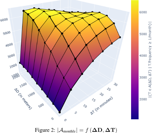
Figure 2 shows the evolution of the number of "Aggregated Travel Requests" that happen at least once a month depending on the values of ∆D and ∆T used in their computation. For example, if we decide to have clusters with a time width ∆T of 5 minutes and a diameter ∆D of 1000 meters we would obtain approximately 4000 distinct space-time clusters. The graph shows that ∆T has overall more impact than ∆D on this metric. We also distinguish an equilibrium between ∆D and ∆T where the number of distinct "Aggregated Travel Requests" that happen at least once a month is maximized. This is logical when considering extreme cases: when both ∆D and ∆T are set to 0 then only travel requests that are exactly the same are aggregated together. This leads to a small number of regular travel requests. On the other hand, when both ∆D and ∆T increases significantly, the number of "Aggregated Travel Requests" itself becomes smaller because travel requests start to be grouped all together in the same clusters.
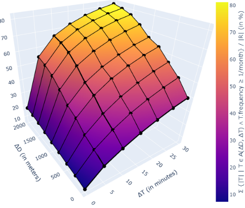
Figure 3: |{r∈T|T∈Amonthly}|
|R|
= f (∆D,∆T)
Additionally, Figure 3 shows the evolution of the proportion of the whole demand represented by the "Aggregated Travel Requests" that happened at least once a month depending on the values of ∆D and ∆T used in their computation. Figure 3 can be viewed as a "weighted" version of Figure 2, where to each cluster is associated a weight proportional to the number of travel requests associated with it. In this case, we can see that if we decide to have clusters with a time width ∆T of 5 minutes and a diameter ∆D of 1000 meters we would cover approximately 40% of the whole set of requests.
Logically, the larger the clusters of travel requests are, the larger the proportion of the demand represented by those travel requests gets. However, we can see that less than half of the whole dataset is depicted by those regular clustered travel requests for most of the low values of ∆D and ∆T.
Consequently, it is clear that "Aggregated Travel Requests" are necessary to be able to describe our historical records in a manageable way: even though they do not completely remove the presence of sparsity and heterogeneity, they drastically reduce their magnitude.
The main question is how should we choose the values of ∆D and ∆T? If our objective was solely to perform a demand prediction, we would probably choose the settings large enough to get nicely preprocessed data. Although, our goal is to provide those "Aggregated Travel Requests" to an optimization model afterwards.
To decide the correct values of ∆D and ∆T, we need to consider the Operational Research model to which those predicted travel requests will be fed.
4 Dial-a-Ride Problem vs. Machine Learning
The Dial-a-Ride Problem is the mathematical model at the core of the optimization frameworks in Demand-Responsive Transport systems [Cordeau and Laporte, 2007; Ho et al., 2018]. The Pick-up and Delivery Problem has several specific constraints consisting of arrivals time windows at the pick-up and drop-off locations, plus a maximum onboard time for each reservation. These are the comfort constraints used to satisfy the travelers with regards to their waiting time and pick-up/drop-off distances. For example, once a traveler has been communicated a pick-up time at 10:00, this timing can be delayed reasonably up to 10:06, but the scheduled transport cannot be too late such as 10:53. Furthermore, customers cannot be kept indefinitely onboard: a deviation can be performed to serve other travelers on the way but it must stay reasonable with regards to the direct travel time without any deviation. In practice, those constraints are what allows the system to insert other travelers and actually group passengers together in the planning of a driver.
More precisely, when a user books a trip from A to B with a departure time at tP , a "Pick-up Time Window" of service is usually designed as follows: [tP -P -, tP +P +] where P - (resp. P +) is the tolerable advance (resp. lateness) to be imposed on the user. In actual services, P - is often close to 0 while P + is often between 10 and 15 minutes.
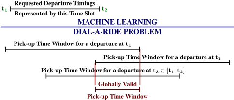
Figure 4 shows how a "Departure Time Slot" of an "Origin-Destination-TimeSlot" Machine Learning model can be converted into a "Pick-up Time Window" of a Dial-a-Ride Problem model. More precisely, in order to build such a time window that can depict any requested departure time within a given "Departure Time Slot" [t1, t2], t1 and t2 should be selected in a way that [t2 -P -, t1 +P +] is a valid temporal interval.
This means that the maximum value for ∆T in our "Aggregated Travel Requests" computation is constrained by the Dial-a-Ride Problem model settings: ∆T ≤ P + + P -.
Using this "Pick-up Time Window", the "Drop-off Time Window" of this travel request from A to B is usually designed based on dtt (A, B) the direct travel time from A to B and mot (A, B) the maximum onboard time from A to B: [tP - P - + s + dtt (A, B) , tP + P + + s + mot (A, B)] where s is the service time associated with this customer.
Figure 5 shows how the geographical clustering also constrains the definition of the "Drop-off Time Window" to use in the Dial-a-Ride Problem model based on the "Pick-up Time Window" defined previously. This constraint comes from the fact that the direct travel time is different between all pairs of departure and destination bus stops.
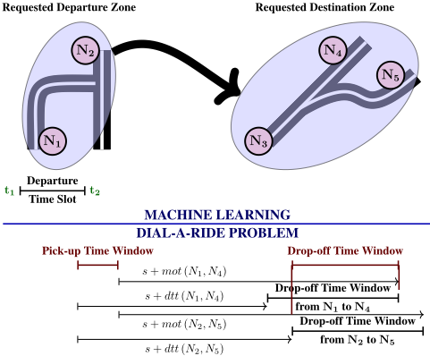
Consequently, we also have to consider the intersection between all of the possible time windows of drop-off. This leads us to define the following constraint in Equation (6) on the "Aggregated Travel Requests" design.
Furthermore, to keep the triangular inequalities valid in the optimization model, the direct travel time from a departure zone to a destination zone must be the maximum direct travel time from any departure to any destination bus stop.
To conclude, we have explained how the Dial-a-Ride Problem, by its mathematical definition, constrains the maximal sizes that we can actually consider for the geographical and temporal clustering steps when preprocessing the data for the Machine Learning model.
In our practical case, we choose ∆D = 500 meters and ∆T = 10 minutes based on the territory configuration. This gives us around 5000 regular "Aggregated Travel Requests" for the Demand Prediction Framework to work with.
5 Demand Prediction Framework
Based on the Data Analysis results presented in Section 3 and the constraints on the Data Aggregation settings explained in Section 4, we can build a matrix of daily "Aggregated Travel Requests". This matrix, noted MA, has 2 dimensions:
- Axis 1: Historical day d, such as March, 18th 2021;
- Axis 2: "Aggregated Travel Requests" that happened at least once a month, such as "From Z4 to Z9 with a departure time between 10:02 and 10:07".
In the cell at line d and column T of MA, we store the ratio between the number of historical travel requests represented by T that happened during d and the total number of travel requests that happened during d. Each line of this matrix thus depicts the probability that a travel request happening a given day belongs to each of those "Aggregated Travel Requests".
It is that line for the next coming day that we aim to predict.
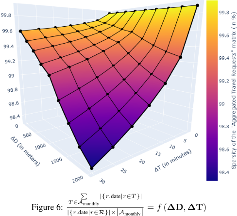
Figure 6 shows the evolution of the sparsity of MA depending on the values of ∆D and ∆T. This is also an important metric when considering that this matrix is used afterwards in the Demand Prediction Framework. It is noticeable that, in any case, sparsity is always an issue, even the largest clustering considered still leads to more than 98% of sparsity which is way higher than what can be found in the literature [Zhuang et al., 2022].
As our time step is the whole day, the size of the Training Set is necessarily limited: 8 years of data, which is the maximum that we dispose of in our case, can only account for roughly 2500 lines of data. Based on this dataset size constraint, we decide to consider two Machine Learning models to build this Demand Prediction Framework.
The first one is a basic Moving Average (MA) model.
The second one is a Long Short-Term Memory (LSTM) model [Hochreiter and Schmidhuber, 1997]. For the latter, we provide additional information about each historical day to enrich the model: position of the year in cosinus and sinus representation, presence of holidays and weather details. We also design a custom trainable Threshold Layer based on the sigmoid function that we add in output of the LSTM model to reduce the noise within its predictions.
To compare the performance of both models, we use all of our dataset as a Training Set except the last month that we use as a Test Set to analyze their generalization capacities.
The input data is always the last 4 weeks of the historical demand that precede the day to predict.
We consider the following metrics to compare ˆMA the output of a Demand Prediction Framework with the ground truth MA extracted from the historical records:
| Model | MSE | PCP | WCP |
|---|---|---|---|
| MA | 4.2E-7 | 74.1% | 27.3% |
| LSTM | 4.6E-7 | 71.5% | 27.6% |
- Mean Squared Error (MSE)
- Proportion of Correct Predictions (PCP)
- Weight of Correct Predictions (WCP)
Those 3 metrics indicate the quality of a prediction with regards to how Machine Learning techniques are usually evaluated (MSE) but also how the rightfully predicted travel requests will be taken into account within the optimization framework (PCP and WCP) as travel requests with higher probability of happening have higher chances to be taken into account within the plannings of the drivers.
Table 1 shows the average values for the three proposed indicators over the complete set of considered case studies. What we can see here is that the MA model detects more correct travel requests but their weight among the incorrect travel requests is lower. Hence, the LSTM model predicts less correct travel requests but give them better probabilities of happening in comparison with what the MA model does.
In both cases, the overall numerical quality of the prediction seems pretty low when we look at those numbers. However, the purpose of this prediction is to be used within an Offline Optimization Algorithm to make space in the initial planning of the vehicles. Consequently, if it is just the global noise that leads us to those values while the predicted travel requests with the highest estimated probabilities of happening and thus the highest weights in the objective function of the optimization scheme are all rightfully predicted travel requests then this could actually be fine.
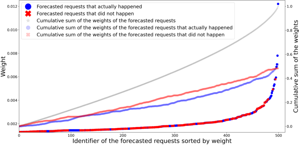
Figure 7 shows an example of how the weights of the predicted travel requests are balanced across the 500 predicted travel requests with the highest probability of happening according to the MA model for the service of February, 12th 2023. We scale those weights so that their sum is equal to 1 to simplify reading. In this specific example, we have PCP = 76.5% and WCP = 36.2% when we consider the complete prediction but PCP = 21.9% and WCP = 51.7% when we consider only the top 500 predicted travel requests. Furthermore, when we compare the weights of the predicted travel requests that are associated with a historical travel request that happened during that day (in blue circles) with the ones of the other predicted travel requests that can be considered as false positives (in red crosses), we can see here that most of the top predicted travel requests are in fact good predictions.
Hence, even though a lot of predicted travel requests are not interesting to us, their weights are actually low and we could simply cut the prediction at a high enough level to consider as few of them as possible.
In the end, even though we have a lot of noisy wrongfully predicted travel requests in output of both Demand Prediction Frameworks, they are still able to put forward rightfully predicted travel requests in terms of estimated probability of happening, which should be enough for the Offline Optimization Process. We decide to use the output of the LSTM-based model in the optimization phase as the best ranked travel requests are more often rightfully predicted than in the output of the MA model.
6 Look-ahead Offline Optimization Process
Our work targets the optimization of the plannings of the drivers at the start of the day in a dynamic context where new travel requests will happen during their shifts. Various approaches to tackle this problem have been considered in the "Vehicle Routing Problem" literature: two-stage [Bernardo and Pannek, 2018] and multi-stage stochastic optimization [Saint-Guillain et al., 2015], an objective function based on simulations [Zigrand et al., 2021] as well as adding fake travel requests into the list of travel requests to serve in order to make space in the already validated bookings [Tensen, 2015]. It is on that last idea that we have designed our Look-ahead Offline Optimization Process.
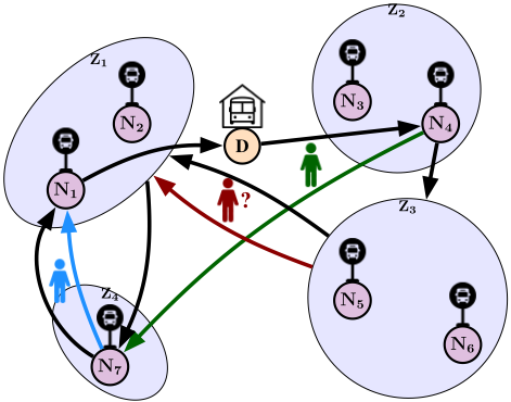
Figure 8 displays why we optimize the initial plannings of the drivers by considering predicted travel requests within their routes. In this example, we design the virtual path of the vehicle in black dotted arrows. In this planning, an in-advance travel request from N4 to N7 and another one from N7 to N1 have been taken into account alongside a predicted travel request from Z3 to Z1. Consequently, this planning allows the driver to perform this trip: D → N4 → {N5,N6} → {N1,N2} → N7 → N1 → D where D is the depot of the vehicle. The actual initial planning is D → N4 →→ N7 → N1 → D but we have made space in that planning so that any travel request represented by the optional one in red in the picture can easily be inserted in the current schedule.
The baseline of our work is the traditional optimization scheme where the Total Duration of the Rides objective function is used in the Offline Optimization Process to rework the plannings of the drivers at the start of the day [Vall´ee, 2019]. Our approach is an optimization scheme where the Look-ahead Offline Optimization Process is used to rework the plannings of the drivers at the start of the day by saturating their routes with the most probable travel requests for the coming day and then removing those virtual stops from their routes. In both cases, the traditional Online Insertion Algorithm based on the Total Duration of the Rides minimization is used the rest of the time to answer the travel requests performed by customers.
We implemented a Dynamic Dial-a-Ride Problem solver based on a Combinatorial Benders Decomposition [Codato and Fischetti, 2006] inspired by recent publications on Vehicle Routing Problems [Fachini and Armentano, 2020] and the Selective Dial-a-Ride Problem [Riedler and Raidl, 2018]. This solver follows a "cluster-first, route-second"
approach where a Master Problem dispatches travel requests to available vehicles while Subproblems, one per vehicle, are responsible for checking the feasibility of these assignments. This decomposition approach allows us to obtain optimal solutions for medium-sized instances, up to a few hundred travel requests, and good solutions for large-scale instances, up to a thousand travel requests, in reasonable computation time and resources. The objective function is to maximize the expected insertion rate of a given set of start plannings for the drivers. In-advance travel requests must be served while predicted travel requests are optional.
We consider all of the historical days of service of the last month available in our dataset, where between 2000 and 3000 travel requests are performed daily, and run on each one of them the following simulation procedure:
- Optimize the initial plannings of the drivers using either the traditional or the look-ahead approach;
- Simulate the sequential arrival of the historical travel requests into the system as they actually happened;
- Report the proportion of the travel requests that were successfully inserted into the plannings of the drivers.
| Approach | Average Insertion Rate |
|---|---|
| Total Duration of the Rides | 58% |
| Look-ahead | 60% |
| Theoretical Upper Bound | 70% |
On average, our approach was able to answer positively 60% of the travel requests while the traditional approach was able to answer positively 58% of the travel requests, the maximum possible being 70% according to our solver. In other words, we obtain a relative improvement in comparison with current practices of 3.5% and a first step towards closing the gap with regards to the upper bound of what is actually possible to do.
7 Conclusion
In this work we discussed how optimization-driven predictions can be radically constrained in their design by the mathematical model that defines the considered problem. We also provided new numerical insights into the mobility needs of suburban areas and how complicated it is to manage them within a Demand Prediction Framework.
Plugged into an Dynamic Dial-a-Ride Problem solver, we also showed the potential of such a look-ahead approach in terms of improved flexibility for the service.
In the future, we first aim to develop a new online insertion policy that takes advantage of the optimization performed at the start of the day. We also want to improve the Demand Prediction Framework used to feed the solver with potential travel requests to serve.
Acknowledgments
We would like to thank the whole Research and Development Team of Padam Mobility for all the useful discussions as well as their continuous support throughout this project.
@inproceedings{ijcai2023p703,
  title     = {Optimization-driven Demand Prediction Framework for Suburban Dynamic Demand-Responsive Transport Systems},
  author    = {Zigrand, Louis and Wolfler Calvo, Roberto and Traversi, Emiliano and Alizadeh, Pegah},
  booktitle = {Proceedings of the Thirty-Second International Joint Conference on
               Artificial Intelligence, {IJCAI-23}},
  publisher = {International Joint Conferences on Artificial Intelligence Organization},
  editor    = {Edith Elkind},
  pages     = {6335--6342},
  year      = {2023},
  month     = {8},
  note      = {AI for Good},
  doi       = {10.24963/ijcai.2023/703},
  url       = {https://doi.org/10.24963/ijcai.2023/703},
}
TY - CPAPER TI - Optimization-driven Demand Prediction Framework for Suburban Dynamic Demand-Responsive Transport Systems AU - Zigrand, Louis AU - Wolfler Calvo, Roberto AU - Traversi, Emiliano AU - Alizadeh, Pegah T2 - Proceedings of the Thirty-Second International Joint Conference on Artificial Intelligence, IJCAI-23 PB - International Joint Conferences on Artificial Intelligence Organization PY - 2023 SP - 6335 EP - 6342 DO - 10.24963/ijcai.2023/703 UR - https://doi.org/10.24963/ijcai.2023/703 ER -Copied
Machine-readable versions of this paper, for tools and AI agents:





