
A Top-Down Tree Model Counter for Quantified Boolean Formulas
Proceedings of the Thirty-Third International Joint Conference on Artificial Intelligence. Main Track. Pages 1853-1861.
https://doi.org/10.24963/ijcai.2024/205
Keywords
- Constraint Satisfaction and Optimization: CSO: Satisfiabilty
- Constraint Satisfaction and Optimization: CSO: Solvers and tools
Abstract
This paper addresses the challenge of solution counting for Quantified Boolean Formulas (QBFs), a task distinct from the well-established model counting problem for SAT (\#SAT). Unlike SAT, where models are straightforward assignments to Boolean variables, QBF solution counting involves tree models that capture dependencies among variables within different quantifier blocks. We present a comprehensive top-down tree model counter capable of handling diverse satisfiable QBF formulas. Emphasizing the critical role of the branching heuristic, which must consider variables in the correct order according to quantification blocks, we further demonstrate the importance of addressing connected components, free variables, and caching. Experimental results indicate that our proposed approach for counting tree models of QBF formulas is highly efficient in practice, surpassing existing state-of-the-art methods designed for this specific purpose.
- [Audemard et al., 2022] Gilles Audemard, Jean-Marie Lagniez, and Marie Miceli. A new exact solver for (weighted) max#sat. In 25th International Conference on Theory and Applications of Satisfiability Testing, SAT 2022, volume 236 of LIPIcs, pages 28:1-28:20. Schloss Dagstuhl -Leibniz-Zentrum für Informatik, 2022.
- [Aziz et al., 2015] Rehan Abdul Aziz, Geoffrey Chu, Chris- tian J. Muise, and Peter J. Stuckey. #∃sat: Projected model counting. In Theory and Applications of Satisfiability Test- ing -SAT 2015 -18th International Conference, volume 9340 of Lecture Notes in Computer Science, pages 121- 137. Springer, 2015.
- [Balabanov and Jiang, 2012] Valeriy Balabanov and Jie- Hong R. Jiang. Unified QBF certification and its appli- cations. Formal Methods Syst. Des., 41(1):45-65, 2012.
- [Balabanov et al., 2015] Valeriy Balabanov, Jie- Hong Roland Jiang, Mikolas Janota, and Magdalena Widl. Efficient extraction of QBF (counter)models from long-distance resolution proofs. In Proc. of the 29th AAAI Conf. on Artificial Intelligence (AAAI), pages 3694-3701. AAAI Press, 2015.
- [Bart et al., 2014] Anicet Bart, Frédéric Koriche, Jean-Marie Lagniez, and Pierre Marquis. Symmetry-driven decision diagrams for knowledge compilation. In Proc. of 21st Eu- rop. Conf. on Artificial Intelligence (ECAI), volume 263 of Frontiers in Artificial Intelligence and Applications, pages 51-56. IOS Press, 2014.
- [Bauland et al., 2005] Michael Bauland, Elmar Böhler, Na- dia Creignou, Steffen Reith, Henning Schnoor, and Herib- ert Vollmer. Quantified constraints: The complexity of decision and counting for bounded alternation. Electron. Colloquium Comput. Complex., TR05-024, 2005.
- [Becker et al., 2012] Bernd Becker, Rüdiger Ehlers, Matthew Lewis, and Paolo Marin. ALLQBF Solving by Computational Learning. In Proc. of the 10th Int. Conf. on Automated Technology for Verification and Analysis (ATVA), volume 7561 of LNCS, pages 370-384. Springer, 2012.
- [Beyersdorff et al., 2014] Olaf Beyersdorff, Leroy Chew, and Mikolas Janota. On unification of QBF resolution- based calculi. In Proc. of the 39th Int. Symp. on Math- ematical Foundations of Computer Science (MFCS), vol- ume 8635 of LNCS, pages 81-93. Springer, 2014.
- [Beyersdorff et al., 2021] Olaf Beyersdorff, Janota Mikolás, Florian Lonsing, and Martina Seidl. Quantified Boolean Formulas. In Handbook of Satisfiability, volume 336 of Frontiers in Artificial Intelligence and Applications, pages 1177-1221. IOS Press, 2021.
- [Birnbaum and Lozinskii, 1999] Elazar Birnbaum and Eliezer L. Lozinskii. The good old Davis-Putnam procedure helps counting models. J. Artif. Intell. Res., 10:457-477, 1999.
- [Cheng and Jiang, 2023] Che Cheng and Jie-Hong R. Jiang. Lifting (D)QBF preprocessing and solving techniques to (D)SSAT. In Proc. of the 37th AAAI Conf. on Artificial Intelligence (AAAI), 35th Conf. on Innovative Applications of Artificial Intelligence (IAAI), pages 3906-3914. AAAI Press, 2023.
- [Chew and Slivovsky, 2022] Leroy Chew and Friedrich Slivovsky. Towards uniform certification in QBF. In Proc. of the 39th Int. Symp. on Theoretical Aspects of Computer Science (STACS), volume 219 of LIPIcs, pages 22:1-22:23. Schloss Dagstuhl -Leibniz-Zentrum für Informatik, 2022.
- [Dubois, 1991] Olivier Dubois. Counting the number of so- lutions for instances of satisfiability. Theor. Comput. Sci., 81(1):49-64, 1991.
- [Fremont et al., 2017] Daniel J. Fremont, Markus N. Rabe, and Sanjit A. Seshia. Maximum model counting. In Pro- ceedings of the Thirty-First AAAI Conference on Artificial Intelligence, pages 3885-3892. AAAI Press, 2017.
- [Giunchiglia et al., 2021] Enrico Giunchiglia, Paolo Marin, and Massimo Narizzano. Reasoning with quantified boolean formulas. In Handbook of Satisfiability -Second Edition, volume 336 of Frontiers in Artificial Intelligence and Applications, pages 1157-1176. IOS Press, 2021.
- [Goultiaeva et al., 2011] Alexandra Goultiaeva, Allen Van Gelder, and Fahiem Bacchus. A uniform approach for gen- erating proofs and strategies for both true and false QBF formulas. In Proc. of the 22nd Int. Joint Conf. on Artificial Intelligence (IJCAI), pages 546-553. IJCAI/AAAI, 2011. IJCAI
- [Heisinger and Seidl, 2023] Simone Heisinger and Martina Seidl. True crafted formula families for benchmarking quantified satisfiability solvers. In Proc. of the 16th Int. Conf. on Intelligent Computer Mathematics (CICM), vol- ume 14101 of LNCS, pages 291-296. Springer, 2023.
- [Hemaspaandra and Vollmer, 1995] Lane A. Hemaspaandra and Heribert Vollmer. The satanic notations: count- ing classes beyond #P and other definitional adventures. SIGACT News, 26(1):2-13, 1995.
- [Heule et al., 2015] Marijn Heule, Matti Järvisalo, Florian Lonsing, Martina Seidl, and Armin Biere. Clause elimina- tion for SAT and QSAT. J. Artif. Intell. Res., 53:127-168, 2015.
- [Kleine Büning and Bubeck, 2021] Hans Kleine Büning and Uwe Bubeck. Theory of quantified boolean formulas. In Handbook of Satisfiability -Second Edition, volume 336 of Frontiers in Artificial Intelligence and Applications, pages 1131-1156. IOS Press, 2021.
- [Kleine Büning et al., 1995] Hans Kleine Büning, Marek Karpinski, and Andreas Flögel. Resolution for quantified boolean formulas. Inf. Comput., 117(1):12-18, 1995.
- [Ladner, 1989] Richard E. Ladner. Polynomial space count- ing problems. SIAM J. Comput., 18(6):1087-1097, 1989.
- [Lagniez and Marquis, 2017] Jean-Marie Lagniez and Pierre Marquis. On preprocessing techniques and their impact on propositional model counting. J. Autom. Reason., 58(4):413-481, 2017.
- [Lagniez and Marquis, 2019] Jean-Marie Lagniez and Pierre Marquis. A recursive algorithm for projected model count- ing. In Proc. of the 33rd Conf. on Artificial Intelligence (AAAI), 31st Innovative Applications of Artificial Intelli- gence Conf. (IAAI), pages 1536-1543. AAAI Press, 2019.
- [Lagniez and Marquis, 2021] Jean-Marie Lagniez and Pierre Marquis. About caching in d4 2.0. In Workshop on Count- ing and Sampling 2021, 2021.
- [Lagniez et al., 2020] Jean-Marie Lagniez, Emmanuel Lonca, and Pierre Marquis. Definability for model counting. Artif. Intell., 281:103229, 2020.
- [Littman et al., 1998] Michael L. Littman, Judy Goldsmith, and Martin Mundhenk. The computational complexity of probabilistic planning. J. Artif. Intell. Res., 9:1-36, 1998.
- [Lonsing and Egly, 2017] Florian Lonsing and Uwe Egly. Depqbf 6.0: A search-based QBF solver beyond tradi- tional QCDCL. In Proc. of the 26th Int. Conf. on Auto- mated Deduction (CADE), volume 10395 of LNCS, pages 371-384. Springer, 2017.
- [Lonsing and Egly, 2018] Florian Lonsing and Uwe Egly. QRAT+: generalizing QRAT by a more powerful QBF re- dundancy property. In Proc. of the 9th Int. Conf. on Auto- mated Reasoning (IJCAR), volume 10900 of LNCS, pages 161-177. Springer, 2018.
- [Majercik, 2009] Stephen M. Majercik. Stochastic boolean satisfiability. In Armin Biere, Marijn Heule, Hans van Maaren, and Toby Walsh, editors, Handbook of Satisfiabil- ity, volume 185 of Frontiers in Artificial Intelligence and Applications, pages 887-925. IOS Press, 2009.
- [Plank et al., 2023] Andreas Plank, Sibylle Möhle, and Mar- tina Seidl. Enumerative level-2 solution counting for quan- tified boolean formulas (short paper). In Proc. of the 29th Int. Conf. on Principles and Practice of Constraint (CP), volume 280 of LIPIcs, pages 49:1-49:10. Schloss Dagstuhl -Leibniz-Zentrum für Informatik, 2023.
- [Rabe and Tentrup, 2015] Markus N. Rabe and Leander Ten- trup. CAQE: A certifying QBF solver. In Proc. of the Int. Conf. on Formal Methods in Computer-Aided Design (FMCAD), pages 136-143. IEEE, 2015.
- [Sang et al., 2004] Tian Sang, Fahiem Bacchus, Paul Beame, Henry A. Kautz, and Toniann Pitassi. Combining com- ponent caching and clause learning for effective model counting. In Proc. of the 7th Int. Conf. on Theory and Ap- plications of Satisfiability Testing (SAT), Online Proceed- ings, 2004.
- [Sang et al., 2005] Tian Sang, Paul Beame, and Henry A. Kautz. Heuristics for fast exact model counting. In Proc. of the 8th Int. Conf. on Theory and Applications of Satis- fiability Testing (SAT), volume 3569 of LNCS, pages 226- 240. Springer, 2005.
- [Sharma et al., 2019] Shubham Sharma, Subhajit Roy, Mate Soos, and Kuldeep S. Meel. GANAK: A scalable proba- bilistic exact model counter. In Sarit Kraus, editor, Proc. of the 28 Int. Joint Conf. on Artificial Intelligence (IJCAI), pages 1169-1176. ijcai.org, 2019. IJCAI
- [Shaw et al., 2024] Arijit Shaw, Brendan Juba, and Kuldeep S. Meel. An approximate skolem function counter, 2024.
- [Shukla et al., 2019] Ankit Shukla, Armin Biere, Luca Pulina, and Martina Seidl. A survey on applications of quantified Boolean formulas. In Proc. of the Int. Conf. on Tools with Artificial Intelligence (ICTAI), pages 78-84. IEEE, 2019.
- [Shukla et al., 2022] Ankit Shukla, Sibylle Möhle, Manuel Kauers, and Martina Seidl. Outercount: A first-level solution-counter for quantified boolean formulas. In Proc. of the 15th Int. Conf on Intelligent Computer Mathe- matics (CICM), volume 13467 of LNCS, pages 272-284. Springer, 2022.
- [Stockmeyer, 1976] Larry J. Stockmeyer. The polynomial- time hierarchy. Theor. Comput. Sci., 3(1):1-22, 1976.
- [van Bremen et al., 2021] Timothy van Bremen, Vincent Derkinderen, Shubham Sharma, Subhajit Roy, and Kuldeep S. Meel. Symmetric component caching for model counting on combinatorial instances. In Proc. of Thirty-Fifth AAAI Conf. on Artificial Intelligence, pages 3922-3930. AAAI Press, 2021.
- [Wimmer et al., 2019] Ralf Wimmer, Christoph Scholl, and Bernd Becker. The (D)QBF preprocessor HQSpre -un- derlying theory and its implementation. J. Satisf. Boolean Model. Comput., 11(1):3-52, 2019.
References were extracted automatically from the PDF and may contain errors.
Full text extracted automatically from the PDF; figures, tables and equations may differ. The PDF is the version of record.
1 Introduction
Problems of the polynomial hierarchy [Stockmeyer, 1976] emerge in a wide range of applications from artificial intelligence, including reasoning tasks in planning, argumentation, two-player games, formal verification, and synthesis to name a few examples. To handle such problems in a uniform manner, quantified Boolean formulas (QBFs) offer an appealing framework [Shukla et al., 2019] with advanced theory and practice of solving technology [Beyersdorff et al., 2021; Kleine B¨uning and Bubeck, 2021; Giunchiglia et al., 2021].
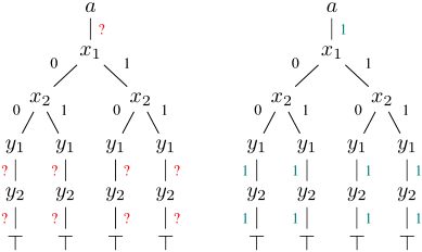
QBFs, extending propositional logic (SAT) by introducing quantifiers over Boolean variables, exhibit notable similarities with SAT. However, the incorporation of universal quantifiers introduces fundamental distinctions. Unlike SAT, a solution to a true QBF is not merely an assignment ensuring the formula's satisfiability. Instead, it takes the form of a tree structure, delineating, for all combinations of universal variable assignments, how existential variables must be set to make the formula evaluate to true. This inherent complexity renders the evaluation of QBFs more intricate compared to SAT. Example 1 provides a concrete illustration of this tree structure.
Example 1. Consider the QBF Φ given by:
This formula has tree models of the structure as shown on the left of Figure 1. On the right, we see a concrete instance of a tree model with concrete values for the existential variables.
The task of a QBF solver is to determine values for the existential variables in a way that each path of the tree encompasses an assignment satisfying the propositional part of the QBF or to demonstrate that no such assignment exists. In the case of the previous example, there exist 80 distinct tree models, signifying that Φ has 80 solutions. These tree models encapsulate crucial information pertaining to the solution of the original reasoning task, such as the plan of a planning problem, an error trace in a verification problem, or the synthesized program in formal synthesis. Consequently, extensive research has been conducted on extracting solutions from QBF solvers [Balabanov and Jiang, 2012; Balabanov et al., 2015; Beyersdorff et al., 2014; Goultiaeva et al., 2011; Chew and Slivovsky, 2022].
In contrast to the extensive exploration of extracting and analyzing solutions in QBFs, the problem of counting the number of solutions, also known as #QBF, has predominantly received theoretical attention [Ladner, 1989; Hemaspaandra and Vollmer, 1995; Bauland et al., 2005]. Some work has delved into counting solutions for QBFs within specific constraints. For instance, in [Shukla et al., 2022], an approach to counting solutions at the outer level was introduced, focusing on a true QBF with the first quantifier block ∃X being existentially quantified. This method enumerates the number of Boolean assignments to variables in X that render the QBF true [Birnbaum and Lozinskii, 1999; Dubois, 1991; Becker et al., 2012]. The enumerative strategy has been extended to the second level, enabling the counting of solutions for true QBFs in the form of ∀X∃Y [Plank et al., 2023]. To achieve this, Skolem functions representing tree models as circuits are incorporated into the formula until the formula evaluates to false. An approximate approach in the related field of Boolean function synthesis will be presented in [Shaw et al., 2024]. However, as of now, there is no approach available that can count solutions for arbitrary QBFs.
It is crucial to distinguish #QBF from classical counting tasks like #SAT, projected model counting [Aziz et al., 2015], (weighted) Max#SAT [Fremont et al., 2017; Audemard et al., 2022], E-MajSAT [Littman et al., 1998], and the stochastic satisfiability (SSAT) [Majercik, 2009] problems. This distinction is notable in the choice of semi-ring for aggregating sub-counts, and the special considerations required for handling connected components, caching, and free variables.
Contributions The principal contribution of this work lies in the development of what, to the best of our knowledge, is the first QBF model counter capable of addressing the counting problem for formulas with arbitrary quantifier prefixes. To this end, we lay the groundwork by establishing the required theoretical foundations and present an efficient implementation. Notably, our approach outperforms existing methods tailored for QBFs with just one quantifier alternation (2QBFs). Through empirical demonstrations, we showcase the prowess of our approach in determining solution counts for instances from diverse formula families, even those considered challenging for contemporary QBF solvers.
2 Preliminaries
We consider quantified Boolean formulas in the form Π.ϕ, where Π = Q1X1 . . .QnXn is referred to as the quantifier prefix (with Qi ∈ {∀, ∃} and Qi ̸= Qi+1 for i ∈ {1, . . . , n - 1}, and X1, . . . ,Xn are pairwise disjoint, nonempty sets of Boolean variables). We denote by Π∃Y the quantifier prefix derived from Π by removing existentially quantified variables that do not belong to Y . For instance, if Π = ∀x1x2∃y1y2∀z1z2∃y3, then Π∃{y1} = ∀x1x2∃y1∀z1z2. Additionally, we use the notation Π \ {x} to represent the quantifier prefix Π with the variable x removed. In the previous example, Π \ {x2} = ∀x1∃y1y2∀z1z2∃y3.
The matrix ϕ is a propositional formula in conjunctive normal form (CNF) over variables Xi. The set Var(ϕ) represents the variables occurring in ϕ. A CNF consists of a conjunction of clauses. Each clause is a disjunction of literals. A literal ℓ is a variable x or the negation ¬x of a variable x. If ℓ is a literal, then Var (ℓ) = x if ℓ = x or ℓ = ¬x. Additionally, ¯ ℓ is defined as x if ℓ = ¬x and ¯ ℓ = ¬x otherwise.
An assignment µ of ϕ is a set of literals over (a subset of) Var(ϕ) such that there is no ℓ ∈ µ with ¯ ℓ ∈ µ. For an assignment µ, Var(µ) = {Var(ℓ) | ℓ ∈ µ}. If Var(µ) = Var(ϕ), then µ is a full assignment, else it is a partial assignment. By 2X we denote the set of all possible assignments to variables in X. Given a propositional formula ϕ and an assign-
Algorithm 1: d4-QBF
input : Φ = Π.ϕ: a QBF formula. output: the number of tree models of Φ. 1 if ϕ is unsat then return 0; 2 (ϕ′ , µ) ← BCP(ϕ); 3 if ∃Qi ∈ Π s.t. Qi = ∀ ∧Xi ∩Var(µ) ̸= ∅ then return 0; 4 if ϕ′ is valid then return CountReduct(Π, ∅, 1); 5 Π′ ← Shrink(Π,Var(ϕ′ )); 6 if cache[ϕ′ ] ̸= ∅ then return CountReduct(Π, Π′ , ϕ′ ); 7 c ← 1; 8 γ ← ConnectedComponent(ϕ′ ); 9 if |γ| > 1 then 10 for ϕ′′ ∈ γ do 11 c ← c × d4-QBF(Π′∃Var (ϕ′′ ) .ϕ′′ ); 12 else 13 v ← selectVar(X′1 ); 14 c1 ← d4-QBF(Π′ \ {v}.ϕ′|v ); 15 c2 ← d4-QBF(Π′ \ {v}.ϕ′|¬v ); 16 c ← (Q′1 = ∀)?c1 × c2 : c1 + c2; 17 cache[ϕ′ ] ← c; 18 return CountReduct(Π,Π′ , c);ment µ, then ϕ|µ denotes the formula obtained when setting all literals x ∈ µ to true and all literals ¬x ∈ µ to false, respectively. For setting a single variable x to true (resp. to false) in a CNF ϕ, we write ϕ|x (resp. ϕ|¬x). A QBF ∃xΠ.ϕ is true iff Π.ϕ|x or Π.ϕ|¬x is true. A QBF ∀xΠ.ϕ is true iff Π.ϕ|x and Π.ϕ|¬x are true. Because of this semantics, a prefix Π = Q1X1 . . . QnXn of QBF Π.ϕ induces an ordering on the variables: xi <Π xj if xi ∈ Xi, xj ∈ Xj and i < j.
A model for a QBF Φ = Π.ϕ with |Var (Φ)| = m is a tree of height m+1 such that every node at level k ∈ {1, . . . ,m} is labeled with a variable xk in the order of the prefix, i.e., if variable xj is at level j and variable xk is at level k with j ≤ k then xj ≤Π xk. The order of the variables from the same quantifier block X can be chosen in an arbitrary manner. We consider two tree models that only differ in the order of variables from the same quantifier block as equal. A node at level k has one child if xk ∈ Xi with Qi = ∃, and two children if xk ∈ Xi with Qi = ∀. We denote the number of different QBF models of a QBF Φ by #(Φ). For instance, for QBF Φ from Example 1, we observe that #(Φ) = 80.
3 A Top-Down QBF Counter
3.1 Algorithm
Below, we present our algorithm, referred to as d4-QBF, aimed at computing the count of tree models for a given QBF. The algorithm is depicted in Algorithm 1. Specifically, it commences by evaluating several base cases (lines 1-6). Initially, it checks if the formula ϕ, the matrix of the QBF Φ, is unsatisfiable by invoking a SAT solver. If the formula is unsatisfiable, then the number of tree models is 0, and the function returns this value (Line 1). Subsequently, the algorithm computes the formula resulting from the Boolean constraint propagation (BCP) procedure by setting literals in clauses of size one to true. The results of BCP are stored in ϕ′ and µ. Here, ϕ′ represents the formula obtained after simplification, and µ signifies the set of unit literals (line 2). Importantly, Var (ϕ′ ) ∩ Var (µ) = ∅, and ϕ ≡ ϕ′ ∧ µ. This transformation does not change the number of tree models, which is an easy consequence of the definition of tree models:
Lemma 1. Let ϕ and ψ be two CNFs on variables X that have the same satisfying assignments over X and let Π be a quantifier prefix s.t. Var (Π) = X. Then #(Π.ϕ) = #(Π.ψ).
If a QBF contains a unit clause with a universal literal, then the QBF is false. Hence, if µ contains a universal literal, the QBF Φ is false, and the function returns 0 (line 3). If ϕ′ is valid, the algorithm computes the number of tree models for Φ directly from Π. This is done using a subroutine CacheReduct whose correctness is proven in Corollary 1.
Finally, the algorithm checks whether ϕ′ , obtained at line 2, has been previously computed by inspecting the cache structure. Notably, cache is a global variable consisting of a hash map associating formulas with natural numbers. However, one has to be careful as it is possible that the same formula is computed twice with different prefixes, inducing different model count. To ensure cache consistency, we define in Section 3.4 a notion of canonical prefix obtained using function Shrink. Inuitively, Shrink removes existential variables that are not in Var(ϕ′ ) and some universal quantified variables as long as they remain on the first quantification block. We give more details in Section 3.4 where we are able to prove that whenever a cache hit occurs, then cache[ϕ′ ] contains the value #(Π′ .ϕ′ ) where Π′ is obtained from Π using Shrink. The function CountReduct then recovers #(Π.ϕ′ ) from this value. Its correctness is proven in Lemma 3.
After addressing all base cases, the algorithm proceeds to the recursive case. The variable c, designated for storing the model count, is initialized to 1 (line 7). Subsequently, the connected components of ϕ are computed in γ utilizing the ConnectedComponent function applied to ϕ′ . This function yields syntactically disjoint sub-formulas of ϕ′ (line 8). As emphasized in Subsection 3.3, this step plays a pivotal role in decomposing the formula's complexity, thereby enhancing the efficiency of the tree model count computation.
Then, once the connected component γ has been computed, we consider two cases based on the size of γ. If |γ| is greater than 1 (line 9), Proposition 1 becomes instrumental. It allows us to compute the tree model count for each sub-formula independently by invoking d4-QBF recursively and then multiplying the results (lines 10-11). To effectively leverage Proposition 1, we adjust the quantifier prefix to include only the existentially quantified variables that are necessary (i.e. Π′∃Var(ϕ′ ) , see Subsection 3.3 for more details).
In the scenario where the formula contains only one connected component, a decision variable v is chosen (line 13) among the variables of the first quantifier block using the selectVar function. Subsequently, two recursive calls to d4-QBF are made, corresponding to the two ways of conditioning v in Π′ .ϕ′ (lines 14-15). As elucidated in Theorem 1 (refer to Subsection 3.2 for a detailed explanation of the branching strategy), the synthesis of results involves multiplication when the variable v is universally quantified and addition when v is existentially quantified (see line 16).
Finally, the cache is updated with the computed count associated with Π′ .ϕ′ (line 17). Since the quantification order remains constant throughout the search, using ϕ′ as the key instead of Π′ .ϕ′ suffices as this QBF lacks free variables. The correctness of this approach is proven in Section 3.4. Once ϕ′ is added to the cache, the CountReduct function can be invoked to obtain the correct tree model count (line 18).
3.2 Branching Strategy
Our algorithm operates recursively by progressing through variable branching in the formula and evaluating the resulting sub-formula. As emphasized earlier, accurate counting of tree models requires adherence to the order of variables outlined by the quantifier prefix. In addition to this requirement, it is crucial to compute the precise number of tree models by appropriately aggregating the sub-counts obtained. The subsequent theorem illustrates the method for recombining subcounts based on the type of quantifier used for branching.
Proof. First assume that Q = ∀. By definition, the models of Φ are the set of trees whose root is labeled by x and is connected to two subtrees T0 and T1 such that T0 is a model of Ψ|¬x and T1 is a model of Ψ|x. There are obviously #(Ψ|x)× #(Ψ|¬x) such trees hence #(Φ) = #(Ψ|x) × #(Ψ|¬x).
Now assume Q = ∃. By definition, the models of Φ are the set of trees whose root r is labeled by x. Further, its root r is connected to a subtree T with root r′ such that: if the edge (r, r′ ) is labeled by 0 then T is a model of Ψ|¬x and if it is labeled by 1 then T is a model of Ψ|x. Hence, there are #(Ψ|¬x) models of Φ such that (r, r′ ) is labeled by 0 and #(Ψ|x) models of Φ such that (r, r′ ) is labeled by 1. These models are obviously disjoint since they have a different label for the edge (r, r′ ). Hence #(Φ) = #(Ψ|x) +#(Ψ|¬x).
Example 2 (Example 1 cont'd). Let us analyze the QBF Φ in Example 1. We decompose #(Φ) into the sum of counts for #(Φ|a) and #(Φ|¬a). QBF Φ|a is defined as ∀x1x2∃y1y2.(x1 ∨ y1) ∧ (x2 ∨ y2), while Φ|¬a is defined as ∀x1x2∃y1y2.(x2 ∨y2). Branching on the variable x2 in Φ|¬a results in #(Φ|¬a) = #((Φ|¬a)|x2 ) × #((Φ|¬a)|¬x2 ). As #((Φ|¬a)|x2 ) = #(∀x1∃y1y2.⊤) = 16 (refer to Example 5 for details) and #((Φ|¬a)|¬x2 ) = #(∀x1∃y1.⊤) = 4, we obtain #(Φ|¬a) = 64. Later, in Example 3, we will demonstrate that #(Φ|a) = 16. Notably, we observe that the correct tree model count is achieved, totaling 16 + (4 × 16) = 80.
If Φ = QX.Ψ, the order of the variables in X can be rearranged without affecting the model count for Φ. Thus, Theorem 1 holds for any variable x ∈ X. This property is utilized by the selectVar heuristic on Line 13 in Algorithm 1. In practice, we employ the same heuristics as cachet [Sang et al., 2004], i.e VSADS [Sang et al., 2005], striving to partition the formula's matrix into connected components for leveraging Proposition 1.
3.3 Connected Components
This optimization is a generalization exploited in many topdown model counters, such as D4 [Lagniez and Marquis, 2019]: decomposability. At its core, decomposability is a property of a CNF formula. A CNF formula ϕ(X) over variables X is deemed decomposable if there exists a partition X1, . . . , Xk of X such that ϕ(X) = ϕ1(X1) ∧ · · · ∧ϕk(Xk). In this case, it is evident that #(ϕ) = ∏ki=1 #(ϕi). Extending this property, we generalize it to estimate the number of models of QBF whose matrix is decomposable:
Proposition 1. Let Φ be a QBF of the form ∀X1∃Y1 . . . ∀Xk∃Yk.ϕ1 ∧ ϕ2 such that X = ⊎ki=1 Xi, Y = ⊎ki=1 Yi and Var(ϕ1) ∩ Var(ϕ2) ⊆ X. We define Y 1 i = Yi ∩Var(ϕ1) and Y 2 i = Yi ∩Var(ϕ2). Then #(Φ) = #(Φ1) × #(Φ2) where Φ1 = ∀X1∃Y 1 1 . . . ∀Xk∃Y 1 k .ϕ1 and Φ2 = ∀X1∃Y 2 1 . . . ∀Xk∃Y 2 k .ϕ2.
Proof. The proof is by induction on the number k of blocks of universal quantifiers. First, assume that k = 0, that is, there is no block of universal quantifiers. In other words, Φ = ∃Y.ϕ1 ∧ ϕ2. In this case, #(Φ) is the number of models of ϕ1 ∧ ϕ2 which is equal by definition to the propositional model count #SAT(ϕ1 ∧ ϕ2), which, by what precedes, is equal to #SAT(ϕ1) × #SAT(ϕ2). But again by definition, #SAT(ϕi) = #(Φi) for i ∈ {1, 2}. Hence #(Φ) = #(Φ1)×#(Φ2) which establishes the base case of the induction. Now assume Φ = ∀X1∃Y1 . . . ∀Xk+1∃Yk+1.ϕ1 ∧ ϕ2. By recursively applying Theorem 1, we have:
Now, observe that for every A1 ∈ 2X1 and E1 ∈ 2Y1 :
where E1 1 (resp. E2 1 ) is defined as E1 restricted to variables in Y 1 1 (resp. Y 2 1 ). For a QBF Φ with fewer than k universal quantifier blocks, by induction, we have #(Φ|A1,E1 ) = #(Ψ1) × #(Ψ2), where Ψi = ∀X2∃Y i 2 . . . ∀Xk+1∃Y i k+1 .ϕi |A1,Ei1 . Note that Ψi = Φi|A1,Ei1 . Thus, #(Φ|A1,E1 ) = #(Φ1 |A1,E1 1 ) × #(Φ2 |A1,Ep21 ). It follows that #(Φ) =
Example 3 (Example 1 cont'd). Let us reevaluate the formula Φ from Example 1, with a specific focus on the formula Φ|a = ∀x1x2∃y1y2.(x1 ∨ y1) ∧ (x2 ∨ y2) highlighted in Example 2. Notably, this formula comprises two connected components: x1 ∨ y1 and x2 ∨ y2. Applying Proposition 1, we determine that #(Φ|a) = #(∀x1x2∃y1.(x1 ∨ y1)) × #(∀x1x2∃y2.(x2 ∨ y2)) = 4 × 4 = 16.
3.4 Counting Tree Models fromCache
Caching plays a crucial role in cutting-edge model counters [Sang et al., 2004; Lagniez and Marquis, 2021; van Bremen et al., 2021; Bart et al., 2014]. To achieve optimal efficiency, it is essential to incorporate the most pertinent information into the cache structure, thereby maximizing positive hits and minimizing the computational effort to retrieve the tree model count (the cost associated with searching in the hash table).
In propositional model counting considering the matrix alone suffices (due to all variables being existentially quantified). Determining the correct tree model count necessitates considering both the matrix and the quantifier prefix. However, using the quantifier prefix along with the matrix as the key when adding items to the cache could be suboptimal, potentially resulting in an artificial increase in negative hits.
Indeed, a naive caching strategy would involve storing the tree model count for every formula Ψ solved so far by our algorithm. Amore effective strategy is employed, improving the number of cache hits by storing only the model count of a reduced QBF. To illustrate, assume a recursive call is made to count the number of models of Ψ1 = ∀X0∃y∃Z∀x1.ϕ for some CNF formula ϕ that does not depend on variables Z. Assume that a previous recursive call has determined that Ψ0 = ∀X0∃y∀x1.ϕ has N models. A naive caching strategy might overlook the knowledge that #(Ψ0) = N since Ψ1 ̸= Ψ0. However, it can be observed that #(Ψ1) = 22|X0| ·|Z|N.
This observation can be generalized as follows: Given a prefix Π = Q1x1 . . .Qkxk, a subprefix Π′ is a prefix of the form Qi1 xi1 . . .Qip xip with i1 < · · · < ip. That is, Π′ is obtained from Π by removing quantified variables but keeping the order. If Π′ is a subprefix of Π and Y ⊆ Var(Π) \ Var(Π′ ), we denote by Π′ + Y the subprefix obtained by adding again the Y variables in Π, keeping the same order as Π. A prefix Π′ is said to be a reduction of Π if the following hold: let y be the first existentially quantified variable of Π′ . Then every universal variable x that appears after y in Π also appears in Π′ . This notion is interesting because of the following lemma:
Lemma 2. Let Π′ be a reduction of Π such that Var(ϕ) ⊆ Var(Π′ ) and let x be the last variable (for the order induced by Π) of Var(Π) \ Var(Π′ ). Then Π′′ = Π′ + x is a reduction of Π and #(Π′′ .ϕ) = (#(Π′ .ϕ))2 if x is universal and #(Π′′ .ϕ) = 22p #(Π′ .ϕ) if x is existential and if there are p universal variables before x in Π′ .
Proof. We first show that Π′′ is a reduction of Π. By definition, Π′′ is a subprefix of Π. Now if x is universally quantified then by definition, there is no existentially quantified variable before x in Π′ since Π′ is a reduction. Hence Π′′ is a reduction. Now assume x is existentially quantified. Let y be the first existentially quantified variable of Π′ . If x appears after y then y is still the first existentially quantified variable of Π′ and hence since Π′ is a reduction, every universal variable of Π that comes after y are in Π′ hence in Π′′ too hence Π′′ is a reduction. If x comes before y, we have to show that every universal variables of Π that are after x are in Π′′ . Since by definition we choose x to be the last variable of Π \ Π′ , every variable of Π appearing after x are also in Π′′ , hence universal variables too. So Π′′ is a reduction.
Now assume that x is universal. Since Π′′ is a reduction, no existential variable of Π can appear before x in Π′′ . Hence we can apply theorem 1 on x to find that #(Π′′ .ϕ) = (#(Π′ .ϕ|x))(#(Π′ .ϕ|¬x)). But Var(ϕ) ⊆ Var(Π′ ), hence x /∈ Var(ϕ). In other words, ϕ|x = ϕ|¬x = ϕ. Hence #(Π′′ .ϕ) = (#(Π′ .ϕ))2 .
Finally, assume x is existential. Since x /∈ Var(ϕ), ϕ is logically equivalent to ϕ ∧ (x ∨ ¬x). By Proposition 1, #(Π′′ .ϕ) = #(Π′ .ϕ) × #(∀X1∃x∀X2.⊤) where X1 are the universal variables of Π′′ before ∃x and X2 the universal variables after ∃x. An easy induction show that #(∀X1∃x∀X2.⊤) = 22|X1| which concludes the proof.
Applying Lemma 2 iteratively on a reduction Π′ of Π until the prefix are the same leads to an efficient algorithm to compute #(Π.ϕ) knowing #(Π′ .ϕ). The pseudocode for this approach is given in Algorithm 2. We start by collecting Var(Π) \ Var(Π′ ) in the for-loop line 2. We maintain a counter p which is the number of universal quantifier in Π′ preceding the current examined variable. We only increase p if the quantifier is universal and if the variables appears in Π′ . Each time a variable not in Π′ is found, we add its quantifier to L together with the number of preceding universal quantifiers. We then go over the list L in reverse order on line 4 and apply the transformation from Lemma 2 to transform #(Π′ .ϕ) into #(Π.ϕ). We hence have the following lemma:
Lemma 3. Let Π be a quantifier prefix, Π′ a reduction of Π and ϕ a CNF formula such that Var (ϕ) ⊆ Var (Π′ ). Then Algorithm 2 on parameters (Π, Π′ , #(Π′ .ϕ)) returns #(Π.ϕ).
Before explaining our caching strategy, we need a last notion. To maximize the number of cache hit, we would like to reduce the prefix of a QBF as much as possible, while still being able to recover the model count. We do this by definining a notion of minimal reduction of a prefix Π as follows: Given a prefix Π and a set of variables V ⊆ Var(Π), define Shrink(Π, V ) to be the subprefix obtained as follows: first, remove from Π every existential variable that does not appear in V and then, if the remaining prefix starts with a universally quantified block, remove from this block (and only this one) every variable that does not appear in V . One can observe that Shrink(Π, V ) is a reduction of Π. Actually it is the minimal reduction Π′ of Π such that Var(Φ) ⊆ Var(Π′ ) in the following sense:
Lemma 4. Let Π′ be a reduction of Π such that V ⊆ Var(Π′ ). Then Shrink(Π, V ) is a reduction of Π′ . In particular, Shrink(Π, V ) = Shrink(Π′ , V ).
Proof. We show that every variable x of Shrink(Π, V ) are also in Π′ . First assume x is existentially quantified.
Then by definition it is in V . Hence x is also in Π′ . Now let x be a variable that is universally quantified in Shrink(Π, V ). Then first assume there is an existential variable y before it in Shrink(Π, V ). In this case, from what precedes, y is also in Π′ and since Π′ is a reduction, every universal variable of Π after y have to be in Π′ . In particular, x is in Π′ . Now, assume that only universal variables appear before x in Shrink(Π, V ). In this case, x ∈ V by definition of Shrink, hence x appears in Π′ since V ⊆ Var(Π′ ). Hence Shrink(Π, V ) is a reduction of Π′ . We hence also that have Shrink(Π, V ) is a reduction of Shrink(Π′ , V ). But with the same argument, Shrink(Π′ , V ) is also a reduction of Shrink(Π, V ). Hence Shrink(Π, V ) = Shrink(Π′ , V ).
We are now ready to explain our caching method. We maintain a cache mapping CNF formula to an integer defined as follows: we let Π0 be the prefix used in the very first call of Algorithm 1. Then for every CNF formulas ϕ such that cache[ϕ] ̸= ∅, we maintain the invariant that cache[ϕ] = #(Π.ϕ) where Π = Shrink(Π0, Var(ϕ)). We maintain also the invariant that every recursive call of Algorithm 1 on Πϕ is such that Π is a reduction of Π0.
Upon these invariants, line 6 of Algorithm 1 returns the correct value. Indeed, by Lemma 4, Π′ = Shrink(Π,Var(ϕ′ )) is equal to Shrink(Π0,Var(ϕ′ )) and by Lemma 3, CountReduct(ϕ′ ,Π,Π′ ) returns #(Π.ϕ′ ) which is equal to #(Π.ϕ) by Lemma 1.
It is now easy to check that both invariants hold at each recursive call. Indeed, every recursive call either removes the first variable of Π′ (lines 14 and 15), which transforms a reduction of Π0 to another reduction of Π0. Or it removes existential variables that do not appear in the formula (line 11) which also produces a reduction of Π0 again.
Finally, when the cache is modified on line 17, the value stored for ϕ′ is equal to #(Π′ .ϕ′ ) where Π′ = Shrink(Π,Var(ϕ′ )) by Theorem 1 and Proposition 1. By Lemma 4 Π′ = Shrink(Π0,Var(ϕ′ )). Hence cache[ϕ′ ] is set to the desired value.
Example 4 (Example 1 cont'd). Let us revisit the formula Φ from Example 1, assuming our initial focus is on counting the ¬a branch. Subsequently, x2 ∨ y2 is incorporated into the cache with a count of 2. It is important to note that the relevant quantifier prefix under consideration here is Π′ = ∀x2∃y2, distinct from the broader Π = ∀x1x2∃y1y2. One can observe that Π′ is a reduction of Π. Hence we can iteratively apply Lemma 2 to retrieve #(Π.ϕ|¬a) from #(Π′ .ϕ|¬a). The former value is hence equal to (221 #(Π′ .ϕ|¬a))2 by applying Lemma 2 first on y1 and then on x1. By observing that #(Π.′ϕ|¬a) = 2, we hence deduce that #(Π.ϕ|¬a) = 64 which can be verified to be the correct model count.
3.5 Counting Tree Models of Valid QBF Formula
When Algorithm 1 is called on a formula whose matrix is a valid CNF formula, then we can explicitly compute the number of tree models using Algorithm 2 and the right parameters, as follows:
| Algorithm | 2: CountReduct |
|---|---|
| input : Π = Q1x1 . . .Qnxn: a quantifier prefix, Π′ : a reduction of Π, N: an integer output: the number of tree models of Π.ϕ if N = #(Π′ .ϕ) | |
| 1 p ← | 0, L← []; |
| 2 | for i from 1 to n do if xi /∈ Var(Π′ ) then L.append((Qi, p)); else if Qi = ∀ then p ← p + 1; |
| 3 | M ← N, ℓ ← length(L); |
| 4 5 | for i from ℓ to 1 do (Q, p) ← L[i]; if Q = ∀ thenM ←M 2 else M ← 22p · M; return M; |
Corollary 1. Let Π be a quantifier prefix. Then Algorithm 2 on parameters (Π, ∅, 1) returns #(Π.⊤).
Proof. It is immediate from Lemma 3 since ∅ is a reduction of Π for any Π and #(⊤) = 1.
Algorithm 1 uses this connection on line 4 to return the correct number of tree models when the matrix ϕ′ is valid.
Example 5 (Example 1 cont'd). Let us revisit again the formula Φ in Example 1, focusing specifically on the valid formula (Φ|¬a)|x2 ) = ∀x1∃y1y2.⊤ obtained in Example 2. Algorithm 2 is hence called with parameters Π = ∀x1∃y1y2, Π′ = ∅ and N = 1. The first for-loop construct the list L = [(∀, 0), (∃, 0), (∃, 0)]. Then N is modified: the last two elements of L both induce a multiplication of N by 220 = 2 and the first one squares everything. Hence the algorithm returns 42 = 16 achieving the correct count of tree models for the given formula.
4 Experimental Evaluation
We implemented the algorithm introduced above in a C++ tool called d4-QBF. 1 This tool builds upon the infrastructure provided by the propositional model counter D4 [Lagniez and Marquis, 2019]. 2 With our evaluation, we aim at addressing the following research questions:
RQ1. How does d4-QBF scale in terms of solved instances and runtime?
RQ2. What is the tree model count of challenging benchmarks and how can we ensure correctness of the counting algorithm?
Environment. All experiments were executed on a compute cluster with dual-socket 16 core AMD EPYC 7313 processors with 3.7 GHz and 256 GB main memory. We run all tools on a single core with a timeout of 900 seconds. The memory limit was set to 32GB.
1 https://zenodo.org/records/11153123
2 https://github.com/crillab/d4
| #Vars | #Clauses | #QBlocks | |
|---|---|---|---|
| KBKFTrue | 8n+1 | 13n+ (n-1) | 2n+2 |
| KBKFTrueTseitin | 8n+1 | 18n | 2n + 2 |
| EQTrueNested | 3n | 2n + 1 | 2n |
| EQTrue | 3n | 2n + 1 | 2 |
| ParityTrue | 2n | 4(n - 1) + 2 | 2 |
Other tools. To the best of our knowledge, currently there exists no model counters for QBFs with arbitrary prefix. For experiments on 2QBFs (QBFs with only quantifier alternation), we run the two tools presented in [Plank et al., 2023]: (1) qcounter, an enumerative solution-counter and (2) baseline, a simple baseline implementation that enumerates all assignments of the universal and calls the propositional model counter Ganak [Sharma et al., 2019]. For evaluating our approach on formulas with more than two quantifier alternations, we run the two QBF solvers Caqe [Rabe and Tentrup, 2015] and DepQBF [Lonsing and Egly, 2017] which are based on orthogonal solving technology and which are top-ranked in the recent QBF competition.
Benchmarks. To evaluate our implementation, we consider seven different families of QBFs originating from two sources:
- Unique-SAT and Random Benchmarks [Plank et al., 2023]. These formulas are true 2QBFs with prefix ∀X∃Y for which the exact model count is known. The random set consists of the 3.950 true instances with 2 ≤ |X|, |Y | ≤ 11. The unique-SAT set consists of 497 formulas that were build from propositional formulas with 26 to 240 variables and 61 to 643 clauses. Given a propositional formula ϕ, the negated unique-SAT QBF encoding based on [Kleine B¨uning et al., 1995] results in a false QBF iff ϕ has exactly one solution. If the propositional formula ϕ contains n variables and has m > 1 models, then the resulting QBF has (2n )2n-m(m-1)m different solutions.
- Crafted instances [Heisinger and Seidl, 2023]. Crafted formula families play an important role in proof complexity. Because of their scalability on a parameter n they provide also expressive benchmarks for testing solvers. Usually, only false instances are considered, but [Heisinger and Seidl, 2023] presented the true formula families KBKFTrue and ParityTrue that were also part of the QBFGallery 2023. 3 In addition to these two families, we introduce three more families: KBKFTrueTseitin, EQTrue, EQTrueNested. Therefore, we extended the generator of [Heisinger and Seidl, 2023]. Properties of the formulas are shown in Table 1. Whereas ParityTrue and EqTrue are 2QBFs, KBKFTrue, KBKFTrueTseitin, and EQTrueNested have n quantifier alternations (where n is the parameter of each specific instance). For our experiments, we chose n ∈ {1, . . . , 25}.
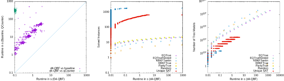
Analysis of RQ1 We compared the runtimes of d4-QBF and the 2QBF solution counters baseline and qcounter on all 2QBF benchmarks (UniqueSAT, Random, ParityTrue, and EQ). The results are shown in the left plot of Figure 2. Our tool d4-QBF solved all of the considered 2QBFs considerably faster than the two other tools. Without the optimizations presented above, our algorithm corresponds to the approach implemented in baseline. The runtimes give a clear empirical indication of the positive impact of the proposed optimizations on the solving performance.
The runtimes of d4-QBF for all considered benchmark sets are shown in the middle of Figure 2. Out of 2586 formulas, only 10 formulas could not be solved (all from the crafted formulas set). As there are currently no other solution counters for QBFs of arbitrary prefix, we run QBF solvers on the crafted formulas. The number of solved formulas are shown in Table 2. Even state-of-the-art solvers could not solve all of the benchmarks. Even more, there are some formulas that are exclusively solved by d4-QBF. These results demonstrate the practical feasibility of tree model counting even for challenging benchmarks.
Analysis of RQ2 The 2QBF benchmarks of [Plank et al., 2023] are generated in such a manner that the number of tree models is known. The formulas of the ParityTrue family have only solution independent of parameter n. Because of their structured nature, we could describe the number of solutions of the other families with (non-linear) recurrences that could be confirmed by d4-QBF. As an interesting side effect, we get some novel insights on the characteristics of the crafted formula families and their solution space. So far, they have mainly been investigated from a proof complexity point of view [Beyersdorff et al., 2021]. The right plot of Figure 2 shows the number of solutions for the instances solved by d4-QBF.
| DepQBF | Caqe | baseline | qcounter | d4-QBF | |
|---|---|---|---|---|---|
| KBKFTrue | 18 | 19 | - | - | 15 |
| KBKFTrueTseitin | 18 | 8 | - | - | 24 |
| EQTrueNested | 24 | 24 | - | - | 24 |
| EQTrue | 24 | 24 | 16 | 6 | 23 |
| ParityTrue | 24 | 18 | 16 | 16 | 24 |
5 Conclusion and Perspectives
In this paper, we addressed the intricate problem of counting solutions for QBFs. Our primary contribution is the development of a comprehensive top-down tree model counter, named d4-QBF, specifically crafted to proficiently handle true QBFs with arbitrary quantifier prefix. Throughout our exploration, we provide the theory to safely incorporate a powerful branching heuristic. Further, we brought attention to the crucial considerations of connected components, free variables, and caching, all of which play key roles in ensuring the efficiency and accuracy of the solution counting process. In addition to being the first counter capable of handling arbitrary QBF formulas, our tool, d4-QBF, distinguishes itself by surpassing state-of-the-art counters specifically designed for 2QBFs. This practical superiority underscores the algorithm's robustness and positions it as a promising solution for solution counting challenges in the domain of QBFs.
Looking forward, our focus is on exploring more tailored simplification techniques to replace propositional Binary Constraint Propagation (BCP) by the QBF version QBCP as employed in [Lonsing and Egly, 2018]. Additionally, we plan to replace the initial SAT call in the algorithm with a strategy customized for QBF formulas. We aim to explore the potential effectiveness of preprocessing techniques [Wimmer et al., 2019; Heule et al., 2015; Cheng and Jiang, 2023], similar to their successful application in solving the #SAT problem [Lagniez and Marquis, 2017; Lagniez et al., 2020]. Another key area for enhancement is the representation of the tree model count, which, at worst, necessitates an exponential number of bits. Our proposed solution involves investigating compact representations, such as polynomial representations, to achieve more efficient modeling.
Acknowledgments
This work has benefited from the support of the National Research Agency under France 2030, MAIA Project ANR-22EXES-0009 and by project ANR KCODA, ANR-20-CE480004. The Institute for Symbolic Artificial Intelligence was in part supported by the LIT AI Lab funded by the State of Upper Austria.
@inproceedings{ijcai2024p205,
  title     = {A Top-Down Tree Model Counter for Quantified Boolean Formulas},
  author    = {Capelli, Florent and Lagniez, Jean-Marie and Plank, Andreas and Seidl, Martina},
  booktitle = {Proceedings of the Thirty-Third International Joint Conference on
               Artificial Intelligence, {IJCAI-24}},
  publisher = {International Joint Conferences on Artificial Intelligence Organization},
  editor    = {Kate Larson},
  pages     = {1853--1861},
  year      = {2024},
  month     = {8},
  note      = {Main Track},
  doi       = {10.24963/ijcai.2024/205},
  url       = {https://doi.org/10.24963/ijcai.2024/205},
}
TY - CPAPER TI - A Top-Down Tree Model Counter for Quantified Boolean Formulas AU - Capelli, Florent AU - Lagniez, Jean-Marie AU - Plank, Andreas AU - Seidl, Martina T2 - Proceedings of the Thirty-Third International Joint Conference on Artificial Intelligence, IJCAI-24 PB - International Joint Conferences on Artificial Intelligence Organization PY - 2024 SP - 1853 EP - 1861 DO - 10.24963/ijcai.2024/205 UR - https://doi.org/10.24963/ijcai.2024/205 ER -Copied
Machine-readable versions of this paper, for tools and AI agents:





