
Convexity Certificates for Symbolic Tensor Expressions
Proceedings of the Thirty-Third International Joint Conference on Artificial Intelligence. Main Track. Pages 1953-1960.
https://doi.org/10.24963/ijcai.2024/216
Keywords
- Machine Learning: ML: Symbolic methods
- Constraint Satisfaction and Optimization: CSO: Solvers and tools
- Machine Learning: ML: Optimization
Abstract
Knowing that a function is convex ensures that any local minimum is also a global minimum. Here, we implement an approach to certify the convexity of twice-differentiable functions by certifying that their second-order derivative is positive semidefinite. Both the computation of the second-order derivative and the certification of positive semidefiniteness are done symbolically. Previous implementations of this approach assume that the function to be minimized takes scalar or vector inputs, meaning that the second-order derivative is at most a matrix. However, the input of many machine learning problems is naturally given in the form of matrices or higher order tensors, in which case the second-order derivative becomes a tensor of at least fourth order. The familiar linear algebra notations and known rules for determining whether a matrix is positive semidefinite are not sufficient to deal with these higher order expressions. Here, we present a formal language for tensor expressions that allows us to generalize semidefiniteness to higher-order tensors and thereby certify the convexity of a broader set of functions.
- [Abadi et al., 2016] Martín Abadi, Paul Barham, Jianmin Chen, Zhifeng Chen, Andy Davis, Jeffrey Dean, Matthieu Devin, Sanjay Ghemawat, Geoffrey Irving, Michael Isard, Manjunath Kudlur, Josh Levenberg, Rajat Monga, Sherry Moore, Derek Gordon Murray, Benoit Steiner, Paul A. Tucker, Vijay Vasudevan, Pete Warden, Martin Wicke, Yuan Yu, and Xiaoqiang Zheng. TensorFlow: A Sys- tem for Large-Scale Machine Learning. In Kimberly Kee- ton and Timothy Roscoe, editors, USENIX Symposium on Operating Systems Design and Implementation (OSDI), pages 265-283. USENIX Association, 2016.
- [Ahmadi and Parrilo, 2013] Amir Ali Ahmadi and Pablo A. Parrilo. A complete characterization of the gap between convexity and sos-convexity. SIAM Journal on Optimiza- tion, 23(2):811-833, 2013.
- [Aho et al., 1986] Alfred V. Aho, Ravi Sethi, and Jeffrey D. Ullman. Compilers: Principles, Techniques, and Tools. Addison-Wesley, 1986.
- [Bach et al., 2023] Francis R. Bach, Elisabetta Cornacchia, Luca Pesce, and Giovanni Piccioli. Theory and ap- plications of the Sum-Of-Squares technique. CoRR, abs/2306.16255, 2023.
- [Blanchard et al., 2020] Pierre Blanchard, Desmond J. Higham, and Nicholas J. Higham. Accurate Computation of the Log-Sum-Exp and Softmax Functions. IMA Journal of Numerical Analysis, 41(4):2311-2330, 08 2020.
- [Cocke, 1970] John Cocke. Global common subexpression elimination. In Robert S. Northcote, editor, Proceedings of a Symposium on Compiler Optimization, pages 20-24. ACM, 1970.
- [Diamond and Boyd, 2016] Steven Diamond and Stephen P. Boyd. CVXPY: A Python-Embedded Modeling Language for Convex Optimization. Journal of Machine Learning Research, 17:83:1-83:5, 2016.
- [Dressler et al., 2019] Mareike Dressler, Sadik Iliman, and Timo de Wolff. An approach to constrained polynomial optimization via nonnegative circuit polynomials and ge- ometric programming. Journal of Symbolic Computation, 91:149-172, 2019.
- [Dressler et al., 2023] Mareike Dressler, Salma Kuhlmann, and Moritz Schick. Geometrical study of the cone of sums of squares plus sums of nonnegative circuits. CoRR, 2305.14848, 2023.
- [Grant and Boyd, 2008] Michael C. Grant and Stephen P. Boyd. Graph implementations for nonsmooth convex pro- grams. In Vincent D. Blondel, Stephen P. Boyd, and Hi- denori Kimura, editors, Recent Advances in Learning and Control, volume 371 of Lecture Notes in Control and In- formation Sciences, pages 95-110. Springer, 2008.
- [Harris et al., 2020] Charles R. Harris, K. Jarrod Millman, Stéfan van der Walt, Ralf Gommers, Pauli Virtanen, David Cournapeau, Eric Wieser, Julian Taylor, Sebastian Berg, Nathaniel J. Smith, Robert Kern, Matti Picus, Stephan Hoyer, Marten H. van Kerkwijk, Matthew Brett, Allan Haldane, Jaime Fernández del Río, Mark Wiebe, Pearu Peterson, Pierre Gérard-Marchant, Kevin Sheppard, Tyler Reddy, Warren Weckesser, Hameer Abbasi, Christoph Gohlke, and Travis E. Oliphant. Array programming with NumPy. Nature, 585:357-362, 2020.
- [Helton and Nie, 2010] J. William Helton and Jiawang Nie. Semidefinite representation of convex sets. Mathematical Programming, 122(1):21-64, 2010.
- [Hickey et al., 2001] Timothy J. Hickey, Qun Ju, and Maarten H. van Emden. Interval arithmetic: From princi- ples to implementation. Journal of the ACM, 48(5):1038- 1068, 2001.
- [Klaus et al., 2022] Julien Klaus, Niklas Merk, Konstantin Wiedom, Sören Laue, and Joachim Giesen. Convexity Certificates from Hessians. In Advances in Neural Infor- mation Processing Systems (NeurIPS), 2022.
- [Klaus et al., 2023] Julien Klaus, Mark Blacher, and Joachim Giesen. Compiling Tensor Expressions into Einsum. In International Conference on Computational Science (ICCS), volume 14074 of Lecture Notes in Computer Science, pages 129-136. Springer, 2023.
- [Laue et al., 2019] Sören Laue, Matthias Mitterreiter, and Joachim Giesen. GENO -GENeric Optimization for Clas- sical Machine Learning. In Advances in Neural Infor- mation Processing Systems (NeurIPS), pages 2187-2198, 2019.
- [Laue et al., 2020] Sören Laue, Matthias Mitterreiter, and Joachim Giesen. A Simple and Efficient Tensor Calcu- lus. In AAAI Conference on Artificial Intelligence (AAAI), pages 4527-4534, 2020.
- [Parrilo, 2000] Pablo Parrilo. Structured semidefinite pro- grams and semialgebraic geometry methods in robustness and optimization. PhD thesis, California Institute of Tech- nology, 2000.
- [Paszke et al., 2019] Adam Paszke, Sam Gross, Francisco Massa, Adam Lerer, James Bradbury, Gregory Chanan, Trevor Killeen, Zeming Lin, Natalia Gimelshein, Luca Antiga, Alban Desmaison, Andreas Köpf, Edward Z. Yang, Zachary DeVito, Martin Raison, Alykhan Tejani, Sasank Chilamkurthy, Benoit Steiner, Lu Fang, Junjie Bai, and Soumith Chintala. PyTorch: An Imperative Style, High-Performance Deep Learning Library. In Hanna M. Wallach, Hugo Larochelle, Alina Beygelzimer, Florence d'Alché-Buc, Emily B. Fox, and Roman Garnett, edi- tors, Advances in Neural Information Processing Systems (NeurIPS), pages 8024-8035, 2019.
References were extracted automatically from the PDF and may contain errors.
Full text extracted automatically from the PDF; figures, tables and equations may differ. The PDF is the version of record.
1 Introduction
Convexity certificates for multivariate differentiable functions have been introduced by Klaus et al. [2022]. Their approach exploits the fact that a twice-differentiable function is convex, if and only if its Hessian, that is, its secondorder derivative, is positive semidefinite (PSD). Convexity of a function can therefore be certified by computing its secondorder derivative and proving that it is PSD. The approach of Klaus et al. [2022] assumes that the function's input is a scalar or a vector. For many machine learning problems, however, it is more natural to express functions not in terms of vectors but higher-order tensors. A simple example is given by the Ising model, a multivariate probability distribution that is given as
where x ∈ X = {0, 1}n and Q ∈ Rn×n is a symmetric parameter matrix. The matrix Q can be learned from m observations x(i) of x by maximizing the log-likelihood function
The symbolic Hessian approach for certifying convexity [Klaus et al., 2022], which assumes that the Hessian is computed as a symbolic function of the input, cannot be applied directly to the log-likelihood function of the Ising model, because its second-order derivative with respect to the input matrix Q is, as for any other function with matrix input, a fourth-order tensor that cannot be expressed in conventional linear algebra notation. Therefore, we generalize the symbolic Hessian approach to functions with tensorial input of any order. To do so, we resort to a tensor expression language based on the einsum notation that we present in Section 3. In addition to the need for a formal tensor language, matrix properties, such as positive semidefiniteness, symmetry, and diagonality, need to be adapted to tensors of arbitrary (even) order. Inferring from the given information that a symbolic tensor expression is positive semidefinite, symmetric, or diagonal becomes more challenging, but also offers new possibilities. We present generalized rules for certifying positive semidefiniteness in Section 4.5. Finally, in Section 5, we evaluate our tensorial extension of the symbolic Hessian approach and show that it is provably more powerful than the approach restricted to vector input, that is, the extension can certify the convexity of a larger class of functions.
An interactive implementation of our tensorial symbolic Hessian approach is available for testing at https://tenvexity. einsum.org.
2 RelatedWork
Traditionally, many functions have been manually proven to be convex. More recently, automatic methods for proving the convexity of certain types of functions have been developed, notably the sum-of-squares (SOS) approach for multivariate polynomials [Helton and Nie, 2010; Ahmadi and Parrilo, 2013; Bach et al., 2023]. A multivariate polynomial is called SOS-convex if its Hessian matrix is an SOS matrix polynomial, which is naturally non-negative. Certifying the SOSconvexity of a polynomial amounts to solving a semidefinite program [Parrilo, 2000].

SOS and extensions, such as sums of non-negative circuit polynomials (SONC) [Dressler et al., 2019; Dressler et al., 2023], work on concrete instances of functions, that is, functions in which every parameter is instantiated by a specific numerical value, whereas symbolic approaches, like the symbolic Hessian approach, certify whole classes of functions. One drawback of the symbolic class-oriented approach is that, even if a class is found to be non-convex, individual instances can still be convex. However, the class-oriented approach has two distinct advantages:
- Certifying convexity symbolically avoids the substantial cost of numerical evaluation. For example, the matrix A in the quadratic form x⊤Ax takes only a few bytes to store as a symbol, but a specific instance can have many entries and thus be extremely large. Processing time differs accordingly. Computing symbolic convexity certificates typically takes only milliseconds.
- Certifying convexity for an entire class of optimization problems also permits to generate efficient solvers for the entire class [Laue et al., 2019]. An alternative but significantly less efficient approach is to transform every new instance from the same problem class into some standard form of a quadratic program (QP), secondorder cone program (SOCP), or semidefinite program (SDP) that can be solved by a solver for the standard form [Grant and Boyd, 2008].
Disciplined convex programming (DCP) is a prominent example of the class-oriented approach that is implemented within CVX [Grant and Boyd, 2008]. The idea of DCP is to combine externally certified atomic functions by using operations that conserve convexity. For instance, a simple DCP rule is that multiplying a convex function with a positive scalar results in another convex function. However, functions that cannot be expressed by using the DCP rules for combining existing atoms cannot be certified as convex. Therefore, the DCP approach is limited by the set of atomic convex functions. Every new atom requires a new, externally computed convexity certificate.
The symbolic Hessian approach by Klaus et al. [2022] avoids these problems for twice-differentiable functions. It certifies convexity of expressions from a formal language that extends standard linear algebra notation by elementwise functions such as log, exp, sin and cos. Here, a convexity certificate for the input function is given by a formal proof that the Hessian of the input is positive semidefinite. A schematic overview of the Hessian approach is given in Figure 1.
So far, the input of the symbolic Hessian approach is limited to functions with vector input, which does not capture naturally occurring examples like the log-likelihood function of the Ising model from the introduction. Here, we generalize the symbolic Hessian approach to higher-order tensors. While the overall procedure for computing convexity certificates remains the same, all its individual steps need to be adapted, which poses various challenges, but also opportunities. In the following sections we explain and resolve the challenges and point out the opportunities.
3 Formal Language
While the log-likelihood function from the introduction can be expressed using standard linear algebra notation, this is not true for its Hessian, which is naturally expressed as a fourthorder tensor. To generalize the symbolic Hessian approach so that it can cope with matrix input, it is necessary to certify even-order tensors as positive semidefinite. To do so, we need a formal language for tensor expressions that subsumes the linear-algebra-based language used by Klaus et al. [2022]. The tensor language can be used to specify the input function as well as all its derivatives, which include its Hessian.
In our context, tensors are mappings from positions to entries. For example, a third-order tensor T ∈ RI×J×K is a mapping
where for any N ∈ N, [N] is the set of positive natural numbers up to N.
The most important operations on tensors are aggregations. In an aggregation, every entry of the result tensor is a sum of products of entries from the operand tensors. For example, a matrix-matrix product is an aggregation between two secondorder tensors. To support tensor aggregations with operand tensors of any order and any number of operands, we use an extended version of the einsum notation that we briefly discuss below.
Furthermore, our tensor-based language also includes common elementwise functions like addition and transcendental functions such as exponentials and logarithms. As a result, the language is rich enough to cover most applications in classical machine learning. Below, we give an overview of our tensor-based language, including our version of the einsum notation. We provide a formal grammar for this language in the supplemental material.
3.1 Tensor-based Language
Input strings are expressions of the form declare <variables> expression <expr>.
For example, the log-sum-exp function
of a matrix A, which is often used as a smooth approximation of the maximum function [Blanchard et al., 2020] and also appears in the concave right part of the loglikelihood function of the Ising model, could be written as declare A 2 expression log(sum(exp(A))). In the following, we use the log-sum-exp function as our running example.
Variable Declaration. The first part of the input string lists all occurring variables followed by their respective order, that is, the number of tensor axes. Since the convexity certifying algorithm works on symbolic expressions, neither the numerical values of the variables nor the lengths of the axes need to be known at any point in the process. However, users can optionally provide additional properties in parentheses. For example,
specifies that the matrix A is symmetric. If the variable declaration is omitted, then we try to deduce the order of A automatically, defaulting to a matrix with no additional properties.
Expressions. The second part of the input string provides the expression that has to be certified as convex. Here, tensor aggregations are written using the einsum notation as described below. Einsum covers anything from simple transpositions to complex aggregations over multiple tensors. In addition, the language supports summation (+) and subtraction (-), special functions for matrices such as det and inv, as well as various elementwise functions such as abs, sign, log, exp, sin and cos. Exponentiation (ˆ) and division (/) are permitted if the right operand is a scalar.
Shorthands. For convenience, our tensor-based language also includes a few optional shortcuts. For example, the logsum-exp function can be expressed succinctly by using the sum keyword, which is short for the sum over all elements in the input tensor. Internally, sum(T) is mapped to the equivalent einsum expression #(i1...io →; T), assuming T is a tensor of order o. The sum-notation is not only simpler and more intuitive, but also invariant to the order of T .
3.2 EinsumNotation
Einsum is a quasi-standard notation for tensor aggregations that is used in popular computational frameworks like NumPy [Harris et al., 2020], TensorFlow [Abadi et al., 2016], and PyTorch [Paszke et al., 2019]. In einsum, tensor aggregations are expressed as operations on indices. For example, A · B #(ij, jk → ik; A,B)
| Operation | Lin. alg. | Einsum |
|---|---|---|
| elementwise prod. inner product outer product matrix transpose matrix diagonal diagonal matrix matrix product | x⊙ y x⊤y xy⊤ A⊤ diag(A) diag(v) A B | #(i, i → i; x, y) #(i, i →; x, y) #(i, j → ij; x, y) #(ij → ji; A) #(ii → i; A) #(i → ii; v) #(ij, jk ik; A,B) |
Table 1: Translation from linear algebra notation to einsum notation.
the matrix product [A · B]ik = ∑j∈[J] AijBjk of A ∈ RI×J and B ∈ RJ×K in einsum notation becomes
The symbol # is necessary to identify einsum expressions within nested einsum expressions.
In general, einsum expressions take the form
where the Ii are the index strings of the operand tensors Ti, and Ir is the index string of the result tensor. The length of an index string is the order of the corresponding tensor. We provide a formal definition of the syntax and semantics of einsum expressions in the supplemental material. Here, the translation of standard linear algebra expressions into einsum notation in Table 1 provides some examples.
4 Certifying Algorithm
The symbolic Hessian approach comprises five steps: Parsing the user's input into an expression DAG (directed acyclic graph), automatic symbolic differentiation of the parsed expression DAG into a symbolic Hessian, simplification of the resulting expression DAG of the Hessian, annotating nodes in the Hessian expression DAG with property labels such as PSD where possible, and deducing labels for unlabeled DAG nodes using label propagation. If the root node of the Hessian expression DAG can be labeled PSD, then the deductions constitute a convexity certificate for the input expression.
4.1 Parsing the Input
For further processing, user input, that conforms to the tensorbased language described in the previous section, is parsed into an expression DAG [Aho et al., 1986], where common subexpressions have been eliminated [Cocke, 1970], that is, every node of the DAG represents a unique subexpression. For a simple example, Figure 2 shows the expression DAG of the log-sum-exp function.

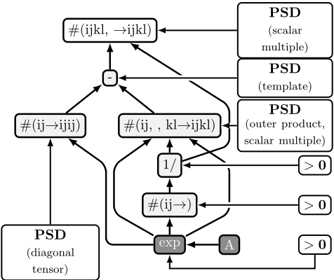
All subsequent steps of the certifying algorithm operate on the expression DAG of the input expression, including the derivation of expression DAGs for the gradient and Hessian of the input expression. The expression DAG of the Hessian of the log-sum-exp function is shown in Figure 3.
4.2 Computing the Hessian
In principle, the simple and efficient tensor calculus by Laue et al. [2020] can be used for computing symbolic Hessians of expressions from our tensor-based language. In practice, however, two challenges remain when differentiating einsum expressions.
The first challenge is posed by duplicate indices in the result index string, that is, expressions of the form #(i → ii; x) that can naturally appear as derivatives. For example, #(ii →; A) is a valid einsum expression that represents the trace of a square matrix A. The derivative of this expression with respect to A is the expression #(i → ii; 1), where 1 represents an all-ones vector. Therefore, we need duplicate output indices in our formal language. However, duplicate output indices are not supported in popular computational frameworks like NumPy or PyTorch.
The second challenge is posed by expressions like #(ij, j →; A, x), whose derivative with respect to the matrix A is #(j → ij; x), which is not a valid einsum expression, because the range of the index i cannot be inferred from the operands, here only the vector x. The range of i is implicitly defined by the matrix A, which is missing from the derivative. We address this challenge by differentiating a different but semantically equivalent expression to #(ij, j →; A, x), namely # (i, ij, j →; 1, A, x), which does not change the result, but the length of the all-ones vector 1 preserves the range of the index i in the derivative, which is #(i, j → ij; 1, x).
4.3 Simplifying Expression DAGs
In the previous section, we took advantage of the fact that syntactically different expressions from the tensor language can be semantically equivalent. In general, however, this is more of a problem, because not all semantically equivalent representations are equivalently well suited for certifying convexity. There are two sources of syntactically sub-optimal representations: First, the user input can include unnecessary operations and vary in the operand order of commutative operations, and second, symbolically computing derivatives of the user input using automatic differentiation systematically creates nested tensor expressions and additional nodes, including, in the very first step, a δ-tensor that generalizes the unit matrix. The δ-tensor nodes are relevant while computing derivatives, but become unnecessary complications afterwards. Therefore, we simplify expressions after every processing step by removing unnecessary nodes from expression DAGs, and by denesting nested tensor expressions into a single expression with a larger number of operands. Denesting can remove intermediary results that are not PSD, which become obstructions when propagating positivity information to the root of the expression DAG of the Hessian.
We illustrate the removal of unnecessary nodes and the denesting of nested tensor expressions on examples involving δ-tensors. The δ-tensor δo of order 2o for some o ∈ N0
has the entry
at every position (i1, ..., io, j1, ..., jo). Notably, δ0 is the scalar value 1 and δ1 is a unit matrix. Aggregations with δtensors are not always trivial operations. The following three examples are different transformations of a matrix A:
All three expressions can be simplified. We do so by applying a sequence of rules that reduce the complexity of an expression without changing its value. For example, the simplification of #(ijkl, kl → ij; δ2, A) is achieved by the following transformations,
where we have applied the transformation rules δsubstitution, where 12 denotes the all-ones matrix, denesting, neutral multiplication, and identity aggregation. All transformation rules together with proofs of correctness are presented in the supplemental material. The second rule, denesting, merges nested expressions into a single but larger expression, thereby avoiding intermediary results. Intermediary results can cause problems in the label propagation phase, where positivity information is propagated through the expression DAG, because nested expressions often include non-PSD intermediary results, even when the whole expression actually is PSD. A small example that illustrates the problem is the linear algebra expression s · xx⊤, where s is a scalar and xx⊤ is the outer product of a vector x. The expression is PSD if s is non-negative. It can be expressed as the following nested einsum expression,
with two non-PSD intermediaries #(i,→ i; x, s) and # (i, j → ij; #(i,→ i; x, s) , 1). The nested expression can be simplified as follows
where we have applied the transformation rules denesting and neutral multiplication. In Section 4.5, we show that the last expression, # (i, , j → ij; x, s, x), can be certified as convex by the certifying algorithm if it is known that s ≥ 0.
4.4 Annotating Nodes in Expression DAGs
At its core the symbolic Hessian approach for certifying convexity propagates positivity information through the expression DAG of the Hessian of the function that has to be certified. If the root node of the DAG of the Hessian can be labeled PSD, then the Hessian is PSD and the input function is convex. Some node labels are either annotated by the user or can be directly inferred from the expression. For instance, the argument of the log-function is always positive, as is the result of the exp-function. Positivity information can then be propagated through the DAG in the label propagation step that we describe in the next section.
We distinguish two types of labels: (1) Property labels, which ensure that a tensor has a certain mathematical property or conforms to a certain shape, and (2) interval labels that ensure that every entry of a tensor is within a given interval.
Property Labels
We use the following property labels: positive semidefinite (PSD), positive definite (PD), negative semidefinite (NSD), negative definite (ND), symmetric (SYM) and diagonal (DIA). We need to generalize these properties, which are typically defined only for matrices, to higher-order tensors.
A tensor T of even order 2o is labeled PSD, if and only if
for any tensor x of order o, which has axes that match those of T in length. The tensor T is labeled NSD, if and only if -T is PSD. Similarly, T is labeled PD, if and only if
for any tensor x of order o and with at least one non-zero entry, which has axes that match those of T in length. The tensor T is labeled ND, if and only if -T is PD. Finally, T is labeled SYM, if and only if
and DIA, if and only if
for all (i1, ..., io) ̸= (j1, ..., jo).
Property annotations for leaf nodes in an expression DAG can be provided as part of the user input, as specified in Section 3. Furthermore, leaf nodes that represent constants are labeled automatically. For example, a square matrix with the same entry in every position is always symmetric.
Interval Labels
In the label propagation phase, we also keep track of the range of a tensor's entries. Knowing the range sometimes allows us to derive property labels. For example, if we know that the range of a scalar s is [0,∞), then when multiplying s with a PSD tensor T, we can deduce that the result tensor s · T is also PSD. Similarly, if the range of s is (-∞, 0], then we can deduce that the result tensor s · T is NSD.
In the label propagation phase, we keep track of a bounding interval for the entries of every tensor subexpression, where tensor subexpressions are represented by nodes of the expression DAG. Subexpressions are intially annotated by the interval (-inf; inf), which can be narrowed down by user input or by functional constraints. For example, log(T) requires that every entry in T is positive, and √T requires that every entry in T is non-negative. A more complex example is given by log(log(T )), which requires that log(T ) > 0 and therefore that every entry in T is larger than 1.
4.5 Propagating Node Labels
Our goal when certifying convexity is to label the root node of the simplified and annotated expression DAG of the Hessian PSD. For this, we can generalize the three basic rules from the vector case. The rules apply locally to nodes in the DAG and their children, and are used to propagate labels, such as PSD, NSD, or SYM, upwards from the leaf nodes to the root node. The three rules read as:
- Outer products #(I, J → IJ; T, T) of a tensor T with itself are PSD.
- The product of a PSD expression with a non-negative scalar is PSD. Multiplying it with a non-positive scalar results in an NSD expression, and similarly for PD, NSD, and ND expressions.
- Elementwise operators can be handled as in the vector case [Klaus et al., 2022], that is, interval annotations can be propagated just as for scalars [Hickey et al., 2001] and property annotations for even-ordered tensors can be propagated as for matrices. For example, the elementwise sum of two PSD tensors is also PSD.
The practical challenge is to represent tensor expressions such that the application of these rules becomes straightforward. We demonstrate the general principle by using the Hessian of the log-sum-exp function as an example, which is shown in Figure 3. The expression not only requires the three basic rules but furthermore serves as an example for applying a more general rule, namely a rule for inferring the label of the difference of a positive diagonal tensor and a PSD tensor, which generalizes from the vector case [Klaus et al., 2022].
We present all propagation rules together with proofs of their correctness in the supplemental material.
The expression DAG of the Hessian of the log-sum-exp function has four nodes that denote einsum operations. The einsum operation at the root multiplies a fourth-order tensor with a scalar. Therefore, the result is PSD if the scalar is nonnegative and the operand tensor is PSD. The einsum operation #(ij → ijij; A) turns a matrix A into a fourth-order diagonal tensor, which is PSD if the matrix A is non-negative, that is, has only non-negative entries. The einsum operation #(ij → ; A) is the same as sum(A), which adds up all entries of the matrix A. If A is non-negative, then the result is a non-negative scalar. The remaining einsum operation, #(ij, , kl → ijkl; A, s, A), is more interesting. It serves as a good example for dealing with einsum expressions with multiple operand tensors.
Expressions with More than Two Operand Tensors
The elementary rules that we use to propagate labels upwards in an expression DAG correspond to either binary or unary tensor operations. For example, simple outer products, multiplication with a scalar, and adding two tensors are binary operations, whereas elementwise functions such as log or exp are unary operations. However, tensor expressions with more than two operand tensors also appear naturally. We deal with einsum expressions with more than two operand tensors by considering a semantically equivalent nested einsum expression in which the outer and all inner einsum expressions are PSD and have at most two operand tensors. For this, we use the same rule set that we use for simplifying expressions. Our example expression #(ij, , kl → ijkl; A, s,A) is semantically equivalent to the nested expression
which is PSD if the scalar is non-negative, because the inner expression #(ij, kl → ijkl; A, A) is an outer product of A with itself and thus PSD, and the outer expression just multiplies the result of the inner expression, which is PSD, with the scalar s.
In Section 4.3 we have claimed that the denested expression #(i, , j → ij; x, s, x) can be certified as PSD for nonnegative scalars s. As in the example from above, this can be shown by nesting the expression into
where the inner expression is also an outer product of a tensor with itself and thus PSD.
It is important to note that in the simplification step we denest expressions to avoid non-PSD intermediary results, because they obstruct label propagation. Here, if possible, we nest expressions such that all intermediary results are PSD. For label propagation, it is sufficient to know that such a semantically equivalent nested expression exists. The actual replacement is not necessary for further processing.
PSD Expression Template
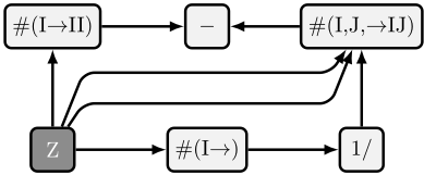
To finish the example of the Hessian of the log-sum-exp function, we still need to discuss the subtraction node that subtracts a PSD tensor from a positive diagonal tensor. In general, the difference of two PSD tensors can be PSD, NSD, or neither. However, differences are provably PSD if they conform to the expression template shown in Figure 4. Klaus et al. [2022] have shown that a similar template applies to many naturally occurring expressions, including the Hessian of the log-sum-exp function, when the basis Z of the template is a vector. In Figure 3 the sub-DAG that correspond to the template is highlighted in light gray, and the sub-DAG that correspond to the basis Z in dark gray, matching Figure 4.
5 Discussion
It is natural to ask what we gain by extending the symbolic Hessian approach beyond vector input. Of course, the tensorial extension subsumes the vector case, that is, any problem with vector input can also be handled by the tensorial extension. The translation from linear algebra language to einsum can even be automated [Klaus et al., 2023]. However, tensorial input can also be flattened into vector input, which can then be addressed by the vectorial symbolic Hessian approach. But flattening tensorial input has three significant disadvantages: First, at the moment it is not clear how to automatize the flattening of input that is naturally given in the form of tensors. Second, there are expressions that can not be flattened symbolically, because knowledge about the length of the tensor axes is necessary, rendering the whole process less general. Examples include the determinant of a matrix, but also practically relevant einsum expressions, such as the interleaving rule# (IK, JL → IJKL; S, T ) ,
which we explain in the supplemental material, for PSD tensors S and T. Third, tensors can have properties, such as symmetry or positive definiteness, that have no natural analog for vectors and which would be lost by flattening. There are expressions that are only PSD when some of the input tensors are defined on restricted domains, for instance, the set of PSD matrices. A prominent example is the function log (det(A)) , which is concave only on the domain of symmetric PSD matrices A.
Additional Property Propagation Rules
A less obvious advantage of the tensorial extension is that it gives us additional rules for propagating properties such as SYM and PSD through an expression DAG on domains that are restricted by these properties.
| Operation | Expression | Convex in | Time (ms) |
|---|---|---|---|
| log-sum-exp | - log(sum(exp(A))) | A | 16.02 ± 0.27 |
| least squares regression | sum((#(ij, i → j; A, x) - y)2 ) | x | 3.01 ± 0.37 |
| UV-decomposition | sum((A - # (ij, kj → ik; U, V ))2 ) | U, V | 4.60 ± 0.38 |
| logdet | - log(det(A)) | A: SYM, PSD | 1.08 ± 0.46 |
| logtrace | - log(trace(A)) | A | 3.00 ± 0.40 |
| exptrace | exp(trace(A)) | A | 12.37 ± 0.38 |
| symmetric trace | trace(# (ia, ij, jb → ab; A, B, A)) | A | 2.51 ± 0.55 |
| Tucker decomposition | sum((X -#(ijk, ia, jb, kc → abc; T,A,B,C))2 ) | A,B,C | 7.00 ± 0.38 |
| rank-1 decomposition | sum((X j, k ijk; u, v,w))2 ) | u, v, w | 5.00 0.34 |
rank-1 decomposition sum((X -#(i, j, k → ijk; u, v,w))2 )
5.00 ± 0.34
Table 2: Examples of convex functions together with their representation in our formal language and running times of the certifying algorithm. Here, sum(T) is a shortcut for # (I →; T ) as explained in Section 3.
Remember that a tensor T is PSD, if and only if
for all tensors X of order o. Therefore, the indices of a PSD tensor T of order 2o always come in pairs (in, jn), n ∈ [o] such that the in-th axis and the jn-th axis of T both correspond to the n-th axis of X. Operations on T that preserve positive definiteness must maintain a pair structure, that is, they can only rearrange, combine, omit or create indices in pairs, but not individually. When an expression is only defined on a restricted domain of tensors, then the PSD condition can be restricted to the same domain. For instance, on the restricted domain of symmetric (and PSD) tensors, the tensor T is PSD if it satisfies the PSD condition for all symmetric (and PSD) tensors X. With this restriction, T may not be PSD in the general sense, but only on the restricted domain. When certifying convexity over such a domain, this leads to two new propagation rules for unary einsum expressions of the form
where T is a PSD tensor and π is a permutation of the four indices i, j, k, l. We show in the supplemental material that the result T ′ is also PSD in the general sense if
π(ijkl) = klij (transposition), or
π(ijkl) = jilk (pair permutation).
We also show that T ′ satisfies the PSD-condition with respect to symmetric matrices X if π(ijkl) = jikl, and that T ′ satisfies the PSD-condition with respect to symmetric PSD matrices X if π(ijkl) = ikjl. A simple counting argument shows that combining the four permutations that maintain positive semidefiniteness with respect to symmetric PSD matrices X results in 24 = 16 out of 4! = 24 permutations on the indices i, j, k and l. A fifth permutation of four indices that can be combined with the existing four permutations can not exist, because 25 > 24. The additional propagation rules generalize from the matrix case (o = 2) to tensors, where these rules swap the indices in four blocks of size o/2 for all even o > 2. The counting argument still holds for rules that permute these four blocks, but further permutations within the blocks remain possible.
Comparison to the Vector Case and to CVX
CVX is, unlike the vectorial Hessian approach as implemented by Klaus et al. [2022], able to certify the concavity of the logdet function. However, to do so, CVXmakes use of an atom specifically for this function. Other functions with similarly restricted domains would need their own atoms. For example, in contrast to the tensorial symbolic Hessian approach, CVXPY (Version 1.4.1) [Diamond and Boyd, 2016] is not able to certify the convexity of the function trace(ABAB), which in einsum notation reads as
for PSD parameter matrices B, and symmetric PSD argument matrices A. To certify the convexity of this function, CVX would need a new atom specifically for this function.
Examples and Computation Time
In Table 2, we list some convex examples from the domain of machine learning together with the time that is needed by our implementation of the tensorial symbolic Hessian approach. The reported computation times are the mean of ten singlethreaded executions, measured on a Windows 11 machine with an AMD Ryzen 9 7900X CPU. Note that running times in the low milliseconds range are brief enough for real-time user interaction.
An interactive version of our implementation can be tested at https://tenvexity.einsum.org.
6 Conclusions
Motivated by optimization problems from machine learning that in their natural formulation feature tensorial, for instance matrix, input, we have generalized the symbolic Hessian approach for certifying convexity of twice-differentiable functions with vector input to tensorial input of arbitrary order. With this extension, we are able to certify the convexity of functions that are defined only on restricted domains, such as log(det(A)), and of functions with input that cannot easily be flattened into a vector.
The extension works for functions that are specified in a formal language of extended tensor expressions. The language is comprehensive enough to cover most areas of machine learning and artificial intelligence. It is also natural in the sense that it is close to standard mathematical notation and does not require externally certified atoms, that is, new symbols, to cover additional functions.
Acknowledgements
This work was supported by the Carl-Zeiss-Stiftung within the project 'Interactive Inference'.
@inproceedings{ijcai2024p216,
  title     = {Convexity Certificates for Symbolic Tensor Expressions},
  author    = {Rump, Paul G. and Merk, Niklas and Klaus, Julien and Wenig, Maurice and Giesen, Joachim},
  booktitle = {Proceedings of the Thirty-Third International Joint Conference on
               Artificial Intelligence, {IJCAI-24}},
  publisher = {International Joint Conferences on Artificial Intelligence Organization},
  editor    = {Kate Larson},
  pages     = {1953--1960},
  year      = {2024},
  month     = {8},
  note      = {Main Track},
  doi       = {10.24963/ijcai.2024/216},
  url       = {https://doi.org/10.24963/ijcai.2024/216},
}
TY - CPAPER TI - Convexity Certificates for Symbolic Tensor Expressions AU - Rump, Paul G. AU - Merk, Niklas AU - Klaus, Julien AU - Wenig, Maurice AU - Giesen, Joachim T2 - Proceedings of the Thirty-Third International Joint Conference on Artificial Intelligence, IJCAI-24 PB - International Joint Conferences on Artificial Intelligence Organization PY - 2024 SP - 1953 EP - 1960 DO - 10.24963/ijcai.2024/216 UR - https://doi.org/10.24963/ijcai.2024/216 ER -Copied
Machine-readable versions of this paper, for tools and AI agents:





