
Improved Parallel Algorithm for Non-Monotone Submodular Maximization under Knapsack Constraint
Proceedings of the Thirty-Third International Joint Conference on Artificial Intelligence. Main Track. Pages 1961-1969.
https://doi.org/10.24963/ijcai.2024/217
Keywords
- Constraint Satisfaction and Optimization: CSO: Constraint learning and acquisition
- Constraint Satisfaction and Optimization: CSO: Applications
- Data Mining: DM: Big data and scalability
- Constraint Satisfaction and Optimization: CSO: Constraint optimization problems
Abstract
This work proposes an efficient parallel algorithm for non-monotone submodular maximization under a knapsack constraint problem over the ground set of size n. Our algorithm improves the best approximation factor of the existing parallel one from 8 to 7 with O(log n) adaptive complexity. The key idea of our approach is to create an alternate threshold algorithmic framework. This new strategy alternately constructs two disjoint candidate solutions within a constant number of sequence rounds. Then, the algorithm boosts solution quality without sacrificing the adaptive complexity. Extensive experimental studies on three applications, Revenue Maximization, Image Summarization, and Maximum Weighted Cut, show that our algorithm not only significantly increases solution quality but also requires comparative adaptivity to state-of-the-art algorithms.
- [Amanatidis et al., 2020] Georgios Amanatidis, Federico Fusco, Philip Lazos, Stefano Leonardi, and Rebecca Reif- fenhäuser. Fast adaptive non-monotone submodular maxi- mization subject to a knapsack constraint. In Annual Con- ference on Neural Information Processing Systems, 2020.
- [Amanatidis et al., 2021] Georgios Amanatidis, Federico Fusco, Philip Lazos, Stefano Leonardi, Alberto Marchetti- Spaccamela, and Rebecca Reiffenhäuser. Submodular maximization subject to a knapsack constraint: Combina- torial algorithms with near-optimal adaptive complexity. In International Conference on Machine Learning, volume 139 of Proceedings of Machine Learning Research, pages 231-242, 2021.
- [Badanidiyuru and Vondrák, 2014] Ashwinkumar Badani- diyuru and Jan Vondrák. Fast algorithms for maximizing submodular functions. In Annual ACM-SIAM Symposium on Discrete Algorithms, pages 1497-1514, 2014.
- [Balkanski and Singer, 2018] Eric Balkanski and Yaron Singer. The adaptive complexity of maximizing a sub- modular function. In Annual ACM SIGACT Symposium on Theory of Computing, pages 1138-1151, 2018.
- [Buchbinder and Feldman, 2019] Niv Buchbinder and Moran Feldman. Constrained submodular maximization via a nonsymmetric technique. Mathematical Operations Research, 44(3):988-1005, 2019.
- [Buchbinder et al., 2015] Niv Buchbinder, Moran Feldman, and Roy Schwartz. Comparing apples and oranges: Query tradeoff in submodular maximization. In Proceedings of the 26th Annual ACM-SIAM Symposium on Discrete Al- gorithms 2015, pages 1149-1168, 2015.
- [Chen and Kuhnle, 2022] Yixin Chen and Alan Kuhnle. Practical and parallelizable algorithms for non- monotone submodular maximization with size constraint. https://arxiv.org/abs/2009.01947, 2022. Link
- [Chen et al., 2019] Lin Chen, Moran Feldman, and Amin Karbasi. Unconstrained submodular maximization with constant adaptive complexity. In Proceedings of the 51st Annual ACM SIGACT Symposium on Theory of Comput- ing, STOC 2019, page 102-113, 2019.
- [Cui et al., 2021] Shuang Cui, Kai Han, Jing Tang, He Huang, Xueying Li, and Zhiyu Li. Streaming algorithms for constrained submodular maximization. Proceedings of the ACM SIGMETRICS conference on Measurement and Analysis of Computer Systems, 6(3):54:1-54:32, 2021.
- [Cui et al., 2023a] Shuang Cui, Kai Han, Jing Tang, He Huang, Xueying Li, and Aakas Zhiyuli. Practical par- allel algorithms for submodular maximization subject to a knapsack constraint with nearly optimal adaptivity. In Thirty-Seventh AAAI Conference on Artificial Intelligence, AAAI 2023, Thirty-Fifth Conference on Innovative Appli- cations of Artificial Intelligence, IAAI 2023, Thirteenth Symposium on Educational Advances in Artificial Intelli- gence, EAAI 2023, Washington, DC, USA, February 7-14, 2023, pages 7261-7269. AAAI Press, 2023.
- [Cui et al., 2023b] Shuang Cui, Kai Han, Jing Tang, He Huang, Xueying Li, Aakas Zhiyuli, and Hanxiao Li. Practical parallel algorithms for non-monotone submodu- lar maximization. CoRR, abs/2308.10656, 2023.
- [Ene and Nguyen, 2019] Alina Ene and Huy L. Nguyen. Submodular maximization with nearly-optimal approxi- mation and adaptivity in nearly-linear time. In Proceed- ings of the Thirtieth Annual ACM-SIAM Symposium on Discrete Algorithms, SODA 2019, San Diego, California, USA, January 6-9, 2019, pages 274-282. SIAM, 2019.
- [Ene and Nguyen, 2020] Alina Ene and Huy L. Nguyen. Par- allel algorithm for non-monotone dr-submodular maxi- mization. In Proceedings of the 37th International Con- ference on Machine Learning, ICML 2020, 13-18 July 2020, Virtual Event, volume 119 of Proceedings of Ma- chine Learning Research, pages 2902-2911. PMLR, 2020.
- [Ene et al., 2019] Alina Ene, Huy L. Nguyen, and Adrian Vladu. Submodular maximization with matroid and pack- ing constraints in parallel. In Proceedings of the 51st An- nual ACM SIGACT Symposium on Theory of Computing, STOC 2019, Phoenix, AZ, USA, June 23-26, 2019, pages 90-101. ACM, 2019.
- [Fahrbach et al., 2019] Matthew Fahrbach, Vahab S. Mir- rokni, and Morteza Zadimoghaddam. Non-monotone sub- modular maximization with nearly optimal adaptivity and query complexity. In Kamalika Chaudhuri and Ruslan Salakhutdinov, editors, Proceedings of the 36th Interna- tional Conference on Machine Learning, ICML 2019, 9- 15 June 2019, Long Beach, California, USA, volume 97 of Proceedings of Machine Learning Research, pages 1833- 1842. PMLR, 2019.
- [Feige et al., 2011a] Uriel Feige, Vahab S. Mirrokni, and Jan Vondrák. Maximizing non-monotone submodular func- tions. SIAM Journal on Computing, 40(4):1133-1153, 2011.
- [Feige et al., 2011b] Uriel Feige, Vahab S. Mirrokni, and Jan Vondrák. Maximizing non-monotone submodular func- tions. SIAM Journal on Computing, 40(4):1133-1153, 2011.
- [Gupta et al., 2010] Anupam Gupta, Aaron Roth, Grant Schoenebeck, and Kunal Talwar. Constrained non- monotone submodular maximization: Offline and secre- tary algorithms. In International Workshop on Internet and Network Economics, 2010.
- [Han et al., 2020] Kai Han, Zongmai Cao, Shuang Cui, and Benwei Wu. Deterministic approximation for submodu- lar maximization over a matroid in nearly linear time. In Advances in Neural Information Processing Systems 33: Annual Conference on Neural Information Processing Sys- tems 2020, NeurIPS 2020, 2020.
- [Han et al., 2021] Kai Han, Shuang Cui, Tianshuai Zhu, En- pei Zhang, Benwei Wu, Zhizhuo Yin, Tong Xu, Shao- jie Tang, and He Huang. Approximation algorithms for submodular data summarization with a knapsack con- straint. Proceedings of the ACM SIGMETRICS confer- ence on Measurement and Analysis of Computer Systems, 5(1):05:1-05:31, 2021.
- [Krizhevsky, 2019] Alex Krizhevsky. Learning multiple lay- ers of features from tiny images. Technical Reports, Uni- versity of Toronto, 2019.
- [Kuhnle, 2021a] Alan Kuhnle. Nearly linear-time, paralleliz- able algorithms for non-monotone submodular maximiza- tion. In Proceedings of the 30th AAAI Conference on Arti- ficial Intelligence 2021, pages 8200-8208, 2021.
- [Kuhnle, 2021b] Alan Kuhnle. Quick streaming algorithms for maximization of monotone submodular functions in linear time. In Proceedings of the 24th International Con- ference on Artificial Intelligence and Statistics 2021, vol- ume 130 of Proceedings of Machine Learning Research, pages 1360-1368, 2021.
- [Lee et al., 2010] Jon Lee, Vahab S. Mirrokni, Viswanath Nagarajan, and Maxim Sviridenko. Maximizing non- monotone submodular functions under matroid or knap- sack constraints. SIAM Journal on Discrete Mathematics, 23(4):2053-2078, 2010.
- [Li et al., 2022] Wenxin Li, Moran Feldman, Ehsan Kazemi, and Amin Karbasi. Submodular maximization in clean lin- ear time. In Advances in Neural Information Processing Systems, pages 7887-7897, 2022.
- [Li, 2018] Wenxin Li. Nearly linear time algorithms and lower bound for submodular maximization. preprint, arXiv:1804.08178, 2018.
- [Mirzasoleiman et al., 2016] Baharan Mirzasoleiman, Ash- winkumar Badanidiyuru, and Amin Karbasi. Fast con- strained submodular maximization: Personalized data summarization. In International Conference on Machine Learning, volume 48 of JMLR Workshop and Conference Proceedings, pages 1358-1367, 2016.
- [Pham et al., 2023] Canh V. Pham, Tan D. Tran, Dung T. K. Ha, and My T. Thai. Linear query approximation algo- rithms for non-monotone submodular maximization under knapsack constraint. In Proceedings of the Thirty-Second International Joint Conference on Artificial Intelligence, IJCAI 2023, 19th-25th August 2023, Macao, SAR, China, pages 4127-4135. ijcai.org, 2023. IJCAI
- [Sun et al., 2022] Xiaoming Sun, Jialin Zhang, Shuo Zhang, and Zhijie Zhang. Improved deterministic algorithms for non-monotone submodular maximization. In Yong Zhang, Dongjing Miao, and Rolf H. Möhring, editors, Computing and Combinatorics -28th International Conference, CO- COON 2022 Proceedings, volume 13595 of Lecture Notes in Computer Science, pages 496-507. Springer, 2022.
References were extracted automatically from the PDF and may contain errors.
Full text extracted automatically from the PDF; figures, tables and equations may differ. The PDF is the version of record.
1 Introduction
A wide range of instances in artificial intelligence and machine learning have been modeled as a problem of Submodular Maximization under Knapsack constraint (SMK) such as maximum weighted cut [Amanatidis et al., 2020; Han et al., 2021], data summarization [Han et al., 2021; Mirzasoleiman et al., 2016], revenue maximization in social networks [Han et al., 2021; Cui et al., 2023a; Cui et al., 2021], recommendation systems [Amanatidis et al., 2021; Amanatidis et al., 2020]. The attraction of this problem comes from the diversity of submodular utility functions and the generalization of the knapsack constraint. The submodular function has a high ability to gather a vast amount of information from a small subset instead of extracting a whole large set, while the knapsack constraint can represent the budget, the cardinality, or the total time limit for a resource. Hence, people are interested in proposing expensive algorithms for SMK these years [Amanatidis et al., 2021; Han et al., 2021; Cui et al., 2023a; Pham et al., 2023; Amanatidis et al., 2020].
∗Corresponding author
Formally, a SMK problem can be defined such as given a ground set V of size n, a budget B > 0, and a nonnegative submodular set function (not necessary monotone) f : 2V ↦→ R+. Every element e ∈ V has its positive cost c(e). The problem SMK asks to find S ⊆ V subject to c(S) = ∑e∈S c(e) ≤ B that maximizes f(S).
One of the main challenges of SMK is addressing big data in which the sizes of applications can grow exponentially. The modern approach is to design approximation algorithms with low query complexity representing the total number of queries to the oracle of f. However, required oracles of f are often expensive and may take a long time to process on the machine within a single thread. Therefore, people think of designing efficient parallel algorithms that can leverage parallel computer architectures to obtain a good solution promptly. This motivates the adaptive complexity or adaptivity [Balkanski and Singer, 2018] to become an important measurement of parallel algorithms. It is defined as the number of sequential rounds needed if the algorithm can execute polynomial independent queries in parallel. Therefore, the lower the adaptive complexity of an algorithm is, the higher its parallelism is.
In the era of big data now, several algorithms that achieve near-optimal solutions with low adaptive complexities have been developed recently (See Table 1 for an overview of low adaptive algorithms). As can be seen, although recent studies make an outstanding contribution by significantly reducing the adaptive complexity of a constant factor approximation algorithm from O(log2 n) to O(logn), there are two drawbacks, including (1) the high query complexities make them become impractical in some instances [Ene and Nguyen, 2020] and (2) there is a huge gap between the high approximation factors of low adaptivity algorithms, e.g. [Amanatidis et al., 2021; Cui et al., 2023a; Cui et al., 2023b], compared to the best one, e.g. [Buchbinder and Feldman, 2019]. This raises to us an interesting question: Is it possible to improve the factor of an approximation algorithm with near-optimal adaptive complexity of O(log n)?
Our contributions. In this work, we address the above question by introducing the AST algorithm for the nonmonotone SMK problem. AST has an approximation factor of 7 + ϵ, within a pair of O(logn) adaptivity, ˜O(nk) query complexity, where ϵ is a constant input. Therefore, our algorithm improves the best factor of the near-optimal adaptive complexity algorithm in [Cui et al., 2023a]. We investigate the performance of our algorithm on three benchmark applications: Revenue Maximization, Image Summarization, and Maximum Weighted Cut. The results show that our algorithm not only significantly improves the solution quality but also requires comparative adaptivity to existing practical algorithms.
| Reference | Approximation Factor | Adaptive Complexity | Query Complexity |
|---|---|---|---|
| [Buchbinder and Feldman, 2019] | 2.6 | poly(n) | poly(n) |
| [Han et al., 2021] | 4 + ϵ | O(n log k) | O(n log k) |
| [Pham et al., 2023] | 4 + ϵ | O(n) | O(n) |
| [Ene et al., 2019] | e + ϵ | O(log2 n) | ˜O(n2 ) |
| [Amanatidis et al., 2021] | 9.465 + ϵ | O(log n) | ˜O(n2 ) |
| [Cui et al., 2023a] (Alg.3) | 8 + ϵ | O(log n) | ˜O(nk) |
| [Cui et al., 2023a] (Alg.5) | 5+2√2+ ϵ ≈ 7.83+ ϵ | O(log2 n) | ˜O(nk) |
| AST (Algorithm 1, this work) | 7+ ϵ | O(log n) | ˜O(nk) |
New technical approach. It is noted that one popular approach to designing parallel algorithms with near-optimal adaptivity of O(logn) is based on making multiple guesses of the optimal solution in parallel and adapting a threshold sampling method 1 , which selects a batch of elements whose density gains, i.e., the ratio between the marginal gain of an element per its cost, are at least a given threshold within O(logn) adaptivity [Amanatidis et al., 2021; Cui et al., 2023a]. By making the guesses of the optimal along with calling the threshold sampling multiple times in parallel, the existing algorithms could keep the adaptive complexity of O(log n) and obtain some approximation ratios.
From another view, we introduce a novel algorithmic framework named "alternate threshold" to improve the approximation factor to 7 + ϵ but keep the same adaptivity and query complexity with the best one [Cui et al., 2023a]. Firstly, we adapt an existing adaptive algorithm to find a nearoptimal solution within O(log n) adaptivity and give a O(1) number of guesses of the optimal solution. Then, the core of our framework consists of a constant number of iterations. It initiates two disjoint candidate sets and then adapts the threshold sampling to upgrade them alternately during iterations: one is updated at odd iterations, and another is updated at even iterations. Thanks to this strategy, we can find the connection between two solutions for supporting each other in evaluating the "utility loss" after each iteration. At the end of this stage, we enhance the solution quality by finding the best element to be added to each candidate's subsets (pre-fixes of i elements) without violating the budget constraint.
It must be noted that our method differs from the Twin Greedy-based algorithms [Han et al., 2020; Pham et al., 2023; Sun et al., 2022], which update both candidate sets at the same iterations but do not allow the integration of the threshold sampling algorithm for parallelization. Besides, we carefully analyze the role of the highest cost element in the optimal solution to deserve more tightness for the problem.
1 We refer to threshold sampling methods as ThreshSeq in [Amanatidis et al., 2021] and RandBatch in [Cui et al., 2023a] with O(log n) adaptivity.
2 RelatedWorks
This section focuses on the related works for the nonmonotone case of the SMK problem.
Firstly, regarding the non-adaptive algorithms, the first algorithm for the non-monotone SMK problem was due to [Lee et al., 2010] with the 5 + ϵ factor and polynomial query complexity. Later, several works concentrated on improving both approximation factor and query complexity [Buchbinder and Feldman, 2019; Gupta et al., 2010; Mirzasoleiman et al., 2016; Li, 2018; Sun et al., 2022; Pham et al., 2023; Han et al., 2021]. In this line of works, algorithm of [Buchbinder and Feldman, 2019] archived the best approximation factor of 2.6 but required a high query complexity; the fastest algorithm was proposed by [Pham et al., 2023] with 4 + ϵ factor in linear queries. For the non-monotone Submodular Maximization under Cardinality (SMC) problem, which finds the best solution that does not exceed k elements to maximize a submodular objective value, the best factor of 2.6 of the algorithm in [Buchbinder and Feldman, 2019] still held. Besides, a few algorithmic models have been proposed for improving running time [Badanidiyuru and Vondr´ak, 2014; Kuhnle, 2021b; Li et al., 2022; Buchbinder et al., 2015]. Among them, the fastest algorithm belonged to [Buchbinder et al., 2015] that provided a e + ϵ factor within O(n log(1/ϵ)/ϵ2 ) queries. However, the above approaches couldn't be parallelized efficiently by the high adaptive complexity of Ω(n).
The adaptive complexity was first proposed by [Balkanski and Singer, 2018] for the SMC problem. Regarding adaptivity-based algorithms for non-monotone SMK, the first one belonged to [Ene and Nguyen, 2019] with e + ϵ and O(log2 n) adaptive complexity. However, due to the high query complexity of accessing, the multi-linear extension of a submodular function and its gradient in their method becomes impractical in real applications [Amanatidis et al., 2021; Fahrbach et al., 2019]. After that, [Amanatidis et al., 2021] devised a (9.465 + ϵ)-approximation algorithm within O(log n), which was optimal up to a Θ(log log(n)) factor by adopting the lower bound in [Balkanski and Singer, 2018]. It is noted that improving the adaptive complexity of a constant factor algorithm from O(log2 n) to O(logn) made an outstanding contribution since it greatly reduced the number of sequential rounds in practical implementation [Cui et al., 2023a; Ene and Nguyen, 2020; Fahrbach et al., 2019]. More recently, [Cui et al., 2023a] created a big step when contributing an efficient parallel one, which resulted in a factor of 8+ϵ within a pair of O(logn) adaptivity and ˜O(nk) query complexity. Nevertheless, this factor still has a huge gap with the best factor of 2.6 [Buchbinder and Feldman, 2019]. They also provided an enhanced version of increasing the approximation factor to 5 + 2√2 + ϵ ≈ 7.83 + ϵ. However, it required a higher adaptivity of O(log2 n). Thus, from this view, the above result of [Cui et al., 2023a] is the best one until now.
People have also focused on developing parallel algorithms for non-monotone SMC these years [Kuhnle, 2021a; Ene and Nguyen, 2020; Fahrbach et al., 2019], etc. The forementioned contributions of [Ene and Nguyen, 2020] was also applied for SMC to get the best approximation factor of e+ϵ, however it used multi-linear extension and thus had a high query complexity. Next, [Kuhnle, 2021a] and [Fahrbach et al., 2019] tried to reduce the adaptive complexity to O(log n) with 25.64+ϵ and 6+ϵ factors. However, [Chen and Kuhnle, 2022] claimed that both [Kuhnle, 2021a] and [Fahrbach et al., 2019] had a non-trivial error because they used the same threshold sampling subroutine which did not work for the non-monotone objective function. [Chen and Kuhnle, 2022] further tried to fixed the previous work and recovered the 6+ϵ factor in O(logn). Recently, [Amanatidis et al., 2021] improved the factor to 5.83 + ϵ in O(logn) adaptivity. Later, the work of [Cui et al., 2023a] archived the factor of 8 + ϵ in O(log n) adaptivity or 4 + ϵ factor in O(log2 n).
After all, our algorithm overcome the existing drawbacks by an improved parallel version with the approximation factor increasing to 7 + ϵ within O(log n) rounds to parallel ˜O(nk) queries.
3 Preliminaries
Given a ground set V = {e1, . . . , en} and an utility set function f : 2V ↦→ R+ to measure the quality of a subset S ⊆ V , we use the definition of submodularity based on the diminishing return property: f : 2V ↦→ R+. f is submodular iff for any A ⊆ B ⊆ V and e ∈ V \ B, we have
Each element e ∈ V is assigned a positive cost c(e) > 0. Let c : 2V ↦→ R+ be a cost function. Assume that c is modular, i.e., c(S) = ∑e∈S c(e) such that c(S) = 0 iff S = ∅.
The problem SMK asks to find S ⊆ V subject to c(S) = ∑e∈S c(e) ≤ B that maximizes f(S). We denote by a tuple (f, V,B) an instance of SMK. Without loss of generality, f is assumed non-negative, i.e., f(X) ≥ 0 for all X ⊆ V and normalized, i.e., f(∅) = 0. We also assume there exists an oracle query, which, when queried with the set S returns the value f(S).
For convenience, we denote by S ∪ e as S ∪ {e}. Next, we denote by O an optimal solution with the optimal value OPT = f(O) and r = argmaxo∈O c(o). We also define the contribution gain of a set T to a set S as f(T|S) = f(T ∪ S) - f(S). Also, the contribution gain of an element e to a set S ⊆ V is defined as f(e|S) = f(S ∪ {e}) - f(S) and f({e}) is written as f(e) for any e ∈ V .
In this paper, we design a parallel algorithm based on Adaptive complexity or Adaptivity, which is defined as follows:
Definition 1 (Adaptive complexity or Adaptivity [Balkanski and Singer, 2018]). Given a value of oracle of f, the adaptivity or adaptive complexity of an algorithm is the minimum number of rounds needed such that in each round, the algorithm makes O(poly(n)) independent queries to the evaluation oracle.
In the following, we recap two sub-problems which our algorithm need to solve: Unconstrained Submodular Maximization and Density Threshold.
Unconstrained Submodular Maximization (UnSubMax) This problem requires to find a subset S ⊆ V that maximizes f(S) without any constraint. The problem was shown NPhard [Feige et al., 2011a].
To obtain mentioned approximation factor, our algorithm adapts the low adaptivity algorithm in [Chen et al., 2019] that achieves an approximation factor of (2 + ϵ) in constant adaptive rounds of O(log(1/ϵ)/ϵ) and linear queries of O(n log3 (1/ϵ)/ϵ4 ).
Density Threshold (DS). The problem receives an instance (f, V, B), a fixed threshold τ and a parameter ϵ > 0 as inputs, it asks to find a subset S ⊆ V satisfies two conditions: (1) f(S) ≥ c(S) · τ ; (2) ∑e∈V \S f(e|S) ≤ ϵ · OPT.
Two algorithms in the literature satisfy the above conditions, including those in [Amanatidis et al., 2021] and [Cui et al., 2023a]. In this work, we adapt the RandBatch algorithm in [Cui et al., 2023a]. RandBatch requires the set I, a submodular function f(·), and parameters ϵ,M to control the solution's accuracy and complexities. RandBatch is combined with the aforementioned density thresholds to set up sieves in parallel for SMK. Due to the space limitations, Pseudocode for RandBatch is given in the appendix.
For an instance (V, f,B) of SMK, two subsets I,M of V , a fixed threshold θ and input parameter ϵ. The performance of RandBatch is provided in the following Lemmas.
Lemma 1 (Lemma 1 in [Cui et al., 2023a]). The sets A, L output by RandBatch(θ, I,M, ϵ, f(·), c(·)) satisfy E[f(A)] ≥ (1 - ϵ)2 θ · E[c(A)] and ϵ · M · ∑u∈L f(u|A) ≤ OPT.
Lemma 2 (Lemma 2 in [Cui et al., 2023a]). RandBatch has O( 1 ϵp (log(|I| · β(I)) +M)) adaptivity, and its query complexity is O(|I|k) times of its adaptive complexity, where β(I) = maxu,v c(u) c(v) . If we use binary search in Line 10 of RandBatch, then it has O( 1 ϵp (log(|I| · β(I)) +M) log(k)) adaptivity, and its query complexity is O(|I|) times of its adaptivity.
Interestingly, we further explore a useful property of RandBatch when applying it to our algorithm.
Lemma 3. The sets A, L output by RandBatch(θ, I,M, ϵ, f(·), c(·)) satisfy E[f(ai|Ai-1)] ≥ (1 - ϵ)2E[c(ai)]θ, where A = {a1, a2, . . . , a|A|},Ai = {a1, a2, . . . , ai}.
4 Proposed Algorithm
In this section, we introduce AST (Algorithm 1), a (7 + ϵ)-approximation algorithm in O(log n) adaptivity and O(n2 log2 n) query complexity.
AST receives an instance (f, V,B), constant parameters δ, ϵ, α as inputs. It contains two main phases. At the first phase (Lines 1-14), it first divides the ground set V into two subsets: V0 contains elements with small costs, and V1 contains the rest. AST then calls ParSKP1 [Cui et al., 2023a] as a subroutine which returns a (1/8 - δ)-approximation solution within O(logn) adaptive rounds. Based on that, the algorithm can offer O(log(1/ϵ)/ϵ) guesses of the optimal solution for the main loop (Lines 4-14). The main loop consists of O(log(1/ϵ)/ϵ) iterations; each corresponds to a guess of the optimal. It sequentially constructs two disjoint solutions, X and Y , one at odd iterations and the other at even iterations. The work of the odd and the even is the same. At the odd (or even) ones, it sets the threshold θX (θY ) and calls the RandBatch routine with the ground set I and the function f(·|X) (f(·|Y )) as inputs to provide the new set Ai (Bi) (Lines 8, 12). It then updates X (Y ) and I as the remaining elements (Line 8 or 12).
The second phase (Lines 15-24) is to improve the quality of solutions. If c(X1 ∪ V0) ≤ ϵB, this phase first adapts UnSubMax algorithm [Chen et al., 2019] for unconstrained submodular maximization over X1 ∪ V0 to get a candidate solution S1 (Lines 15-16). This step is based on an observation that X1 is important in analyzing the algorithm's performance. It then selects the sets of the first i elements added into X and Y and finds the best elements without violating the total cost constraint (Lines 19-24). Finally, the algorithm returns the best candidate solution (Lines 25-26). The details of AST are depicted in Algorithm 1.
At the high level, AST works follow a novel framework that combines an alternate threshold greedy algorithm with the boosting phase. The term "alternate" means that candidate solutions are updated alternately with each other in multiple iterations. At each iteration, only one partial solution is updated based on two factors: one guess of the optimal solution and the remaining elements of the ground set that do not belong to the other solution.
It should be emphasized that the alternate threshold greedy differs from recent works [Cui et al., 2023a; Amanatidis et al., 2021] where two candidate solutions for each guess are constructed after only one adaptive round. Alternate threshold greedy also differs from the twin greedy method in [Han et al., 2020], which allows updating both disjoint sets in each iteration. For the theoretical analysis, the key to obtaining a tighter approximation factor lines in aspects: (1) the connections between X and Y after each iteration of the first loop and (2) carefully considering the role of r to eliminate terms that worsen the approximation factor.
We now analyze the performance guarantees of AST. We consider X and Y after ending the first loop. We first introduce some notations regarding AST as follows.
- Xi , Y i is the set of first i elements added into X and Y , respectively.
Algorithm 1: AST Algorithm
Input: An instance (f, V, B), parameters α, ϵ, δ 1: V0 ← {e ∈ V : c(e) ≤ ϵB/n}, V1 ← V \ V0, I ← V1, p ← 1 2: S0 ←ParSKP1( 1 4 , δ, f(·), c(·)), Γ ← 8αf(S0) (1-8δ)ϵB 3: X ← ∅, Y ← ∅, ∆← ⌈log 1 1-ϵ 8α ϵ2 (1-8δ) ⌉ + 1, M ← 1 ϵ2 ( ∆2 +1) 4: for i = 1 to ∆ do 5: if i is odd then 6: θX ← Γ(1 - ϵ)i 7: (Ai, Ui, Li) ← RandBatch(θX , I , M, p, ϵ, f (·|X), c(·)) 8: X ←X ∪Ai, I ← I \X 9: else 10: θY ← Γ(1 - ϵ)i 11: (Bi, Ui, Li) ← RandBatch(θY , I, M, p, ϵ, f (·|Y ), c(·)) 12: Y ← Y ∪Bi, I ← I \ Y 13: end 14: end 15: For T ∈ {X, Y }, define: Ti is T after the iteration i of the first loop, T i is the set of first i elements added into T . 16: if c(X1 ∪ V0) ≤ ϵB then 17: S1 ←UnSubMax(X1 ∪ V0) 18: end 19: for i = 1 to |X| do 20: ai ← argmaxe∈V :c(Xi∪e)≤B f(Xi ∪ {e}), X′i ← Xi ∪ {ai} 21: end 22: for i = 1 to |Y | do 23: bi ← arg maxe∈V :c(Y i∪e)≤B f (Y i ∪ {e}), Y ′i ← Y i ∪ {ai} 24: end 25: S ← argmaxT∈{X′i }|X| i=1∪{Y ′i }|Y | i=1∪{X,Y,S1} f (T ) 26: return S- Xi and Yi are X and Y after the iteration i of the first loop (Lines 4-14) and X0 = Y0 = ∅.
- O1 is an optimal solution of SMK over instance (f, V1, B).
- For an element e ∈ X ∪ Y , we denote: X<e, Y<e, θX e and θY e as X, Y , θX and θY right before e is selected into X or Y , respectively; l(e) is the iteration when e is added in to X or Y .
Lemma 4 makes a connection between X and Y after each iteration.
Lemma 4. After any iteration i of the first loop (Lines 4-14) of AST, we have:
Proof. Prove a) If i = 1, Y0 = ∅, the Lemma holds. We consider the other case. We divide T into several subsets including T = T2 ∪T4 ∪ . . . ∪Ti-1, where Tj is a set of all elements in T that are added into Yi at iteration j ≤ i-1. Since Tj ⊆ Yi-1 ∩ O1 and c(Xi) ≤ B - c(r) so c(X<e) + c(e) ≤ c(Xi) + c(e) ≤ B for all e ∈ Tj. We therefore classify the elements in Tj into two disjoint sets Tj = T 1 j ∪ T 2 j , where T 1 j = {e ∈ Tj : f(e|X<e) c(e) < θX e , c(X<e) + c(e) ≤ B} and T 2 j = {e ∈ Tj : f(e|X<e) c(e) ≥ θX e , c(X<e)+c(e) ≤ B}. Since (1 - ϵ)θX e = θY l(e)∀e ∈ T 1 j , we have:
where inequality (2) is due to Lemma 1, inequality (4) is due to applying Lemma 3: E[f(e|Y<e)] ≥ (1 - ϵ)2E[c(e)]θY l(e) . It follows that
where inequation (6) is due to the submodularity, inequation (8) is due to setting of M.
Prove b). If i = 2, X1 ∩ O = ∅, the Lemma holds. If i > 2, we only consider set T ⊆ Xi-1 ∩ O′ since we can not bound the f(e|Y<e) if e ∈ X1. We also divide T into subsets: T = T3 ∪ T5 ∪ . . . ∪ Ti-1, where Tj is a set added into Xj at the iteration j ≤ i - 1. We also classify the elements in Tj into two sets Tj = T 1 j ∪ T 2 j , where T 1 j = {e ∈ Tj : f(e|Y<e) c(e) < θY<e , c(Y<e) + c(e) ≤ B} and T 2 j = {e ∈ Tj : f(e|Y<e) c(e) ≥ θY<e , c(Y<e) + c(e) ≤ B}. By a similar argument to the previous case, we have:
which implies that
The proof is completed.
By using Lemma 4, we further provide the bound of f (O′ ∪ T) for T is a subset of X or Y in Lemma 5 when c(r) is very large, i.e., c(r) ≥ (1 - ϵ)B.
Lemma 5. If c(r) ≥ (1 - ϵ)B, one of two following propositions happens
- E[f(S)] ≥ (1 - ϵ)5αOPT.
Similarly, one of two following propositions happens:
When c(X1) < ϵB and c(Y2) < ϵB, it's easy to obtain the approximation factor due to f(S) ≥ max{f(X1), f(Y2)} ≥ ϵBαΓ(1-ϵ)2 . Otherwise, we combine Lemma 5 and the fact that f(O′ ) ≤ f(O′ ∪ X) + f(O′ ∪ Y ) to get the bound of f(O′ ) in Lemma 6. The proofs of them can be found in the Appendix.
Lemma 6. If c(X1) < ϵB and c(Y2) < ϵB, we have:
- If c(r) ≥ (1- ϵ)B, one of two things happens:
Finally, put Lemmata 4,5,6 together and divide O into appropriate subsets, we state the performance's algorithm in Theorem 4.1.
Theorem 4.1. For α = 17 , ϵ ∈ (0, 17 ), δ ∈ (0, 18 ), Algorithm 1 needs O(log n) adaptive complexity and O(nk log2 n) query complexity and returns a solution S satisfying E[f(S)] ≥ (1/7 - ϵ)OPT.
Proof. AST first calls ParSKP1 to find a candidate solution S0. This task takes O( 1δ log( nδ )) adaptivity and O(nk log2 n) query complexity [Cui et al., 2023b]. For the first loop, it calls ThreshSeq ∆ = O( 1ϵ log( 1ϵ )) times. Each time, RandBatch needs O( 1ϵ log( nϵ ) + M) = O( 1ϵ log( nϵ ) + 1 ϵ3 log( 1ϵ )) = O(logn) adaptive complexity and O( nk ϵ log( nϵ ) + nk ϵ3 log( 1ϵ )) = O(nk logn) query complexity. In the second phase, the algorithm may need O( 1ϵ log( 1ϵ )) adaptivity and O( n ϵ4 log3 ( 1ϵ )) query complexity to call UnSubMax algorithm of [Chen et al., 2019] (Lines 16-17). Then, it only has two adaptive rounds and takes O(kn) query complexity to find X′i and Y ′i (Lines 19-24). Therefore, the adaptive complexity of the algorithm is O( 1δ log nδ ) + O( 1ϵ log( 1ϵ ) logn) + O( 1ϵ log( 1ϵ )) + 2 = O(logn) and its query complexity is O(nk log2 n) + O(nk log n) + O( n ϵ4 log3 ( 1ϵ )) +O(nk) = O(nk log2 n). For the approximation factor, we consider the following
cases:
Case 1. If c(X1) ≥ ϵB or c(Y2) ≥ ϵB, we have
Case 2. If c(X1) < ϵB and c(Y2) < ϵB, we have
where inequality (17) is due to the submodularity of f and (V1 \X1) ∩ (V0 ∩X1) = ∅, equality (18) is due to the definition of O′ and inequality (19) is due to applying Algorithm in [Chen et al., 2019]. We now apply Lemma 6 to bound f(O′ ). If c(r) < (1 - ϵ)B, then
Therefore
If c(r) ≥ (1 - ϵ)B, we consider two cases:
- If a) in Lemma 6 happens, then
- If b) in Lemma 6 happens, then
where the inequality (22) is due to ϵM = 1ϵ ( ∆2 +1) > 14 ϵ for ϵ ∈ (0, 17 ), δ ∈ (0, 1 8 ). It follows that
which completes the proof.
5 Experimental Evaluation
This section evaluates our AST's performance by comparing our algorithm with state-of-the-art algorithms for nonmonotone SMK including:
- ParSKP1: The parallel algorithm in [Cui et al., 2023a] that runs in O(log n) adaptivity and returns a solution S satisfying E[f (S)] ≥ (1/8 - ϵ)OPT.
- ParSKP2: The algorithm in [Cui et al., 2023a] that runs in O(log2 n) adaptivity and returns a solution of E[f (S)] ≥ (1/(5 + 2√2) - ϵ) OPT.
- ParKnapsack: The parallel algorithm in [Amanatidis et al., 2021] achieves an approximation factor of (9.465 + ε) within O(log n).
- SmkRanAcc: The non-adaptive algorithm in [Han et al., 2021] that achieves an approximation factor of 4 + ϵ in query complexity of O(n log(k/ϵ)/ϵ).
- RLA: The non-adaptive algorithm in [Pham et al., 2023] with a factor of 4 + ϵ in linear query complexity of O(n log(1/ϵ)/ϵ).
We experimented with the following three applications:
Revenue Maximization (RM). Given a network G = (V,E) where V is a set of nodes and E is a set of edges. Each edge (u, v) in E is assigned a positive weight w(u, v) sampled uniformly in [0, 1] and each node is assigned a positive cost c(u) defined as c(u) = 1 - e√∑(u,v)∈E w(u,v) . The revenue of any subset S ⊆ V is defined as f(S) = ∑v∈V\S √∑u∈S wu,v. Given a budget of B, the goal of the problem is to select a set S with the cost at most B to maximize f(S). As in the prior work, [Amanatidis et al., 2021], we can construct the graph G using a YouTube community network dataset [Han et al., 2021] with 39,841 nodes and 224,235 edges.
MaximumWeighted Cut (MWC). Consider a graph G = (V, E) where each edge (u, v) ∈ E has a non-negative weight w(u, v). For a node subset S ⊂ V , define the weighted cut function f(S) = ∑u∈V \S ∑v∈S w(u, v). The maximum weighted cut problem seeks a subset S ⊆ V that maximizes f(S). As in recent work [Amanatidis et al., 2020], we generate an Erd˝os-R´enyi random graph with 5, 000 nodes and an edge probability of 0.2. The node costs c(u) are randomly uniformly sampled from (0, 1).
Image Summarization (IS). Consider a graph G = (V,E) where each node u ∈ V represents an image, and each edge (u, v) ∈ E has a weight w(u, v) showing the similarity between images u and v. Let c(u) be the cost to acquire image u. The goal is to find a representative subset S ⊆ V under the budget B that maximizes a value f(S) = ∑u∈V maxv∈S wu,v - 1 |V | ∑u∈V ∑v∈S wu,v [Mirzasoleiman et al., 2016; Han et al., 2021]. As in recent works [Han et al., 2021; Mirzasoleiman et al., 2016], we create an instance as follows: First, randomly sample 500 images from the CIFAR dataset [Krizhevsky, 2019] of 10,000 images, then measure the similarity between images u and v using the cosine similarity of their 3,072-dimensional pixel vectors.
Experiment setting. In our experiments, we set the accuracy parameter ϵ = 0.1 for all algorithms evaluated, and for AST, we set δ = 0.12. We used OpenMP to program with C++ language. Besides, we experimented on a high-performance computing (HPC) server cluster with the following parameters: partition=large, #threads(CPU)=128, node=4, max memory = 3,073 GB. For UnSubMax, we use setting of previous works [Amanatidis et al., 2021; Cui et al., 2023a], i.e, we adapt Algorithm in [Feige et al., 2011b] returning 1/4-ϵ ratio in one adaptive round and O(n) query complexity.
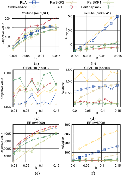
Experimental Result. In Figures 1(a), (c), and (e), we compare the objective values between different algorithms. The results show that our AST achieves the best objective values for both the RM and MWC applications. In RM, the objective values achieved by RLA, SmkRanAcc, and ParSKP1 are the same, ParKnapsack attains lower objective values while ParSKP2 hits the lowest objective values among the algorithms. Especially, our one marks the highest value when B = 0.015, about 1.3 times higher than the others in RM. In IS, ParKnapsack reaches the highest values while ParSKP2 hits the lowest. Our algorithm results in best values at some points and drops at others. As shown in Figure 1 (c), most algorithms fluctuate widely. The variation in the quality of these algorithms might be due to the characteristics of this dataset.
In Figures 1(b), (d), and (f), we make the comparisons about the number of adaptive rounds. The results show that SmkRanAcc and RLA always require the highest number of adaptive rounds across all three applications. For the AST, the number of adaptive rounds is equivalent to ParSKP1 for RM and MWC. Besides, for IS, the adaptive number of rounds for AST is higher than that of ParSKP1, which has the lowest number of rounds. However, the higher number in this case is insignificant. Overall, our algorithm outperforms the others in both solution performance and the quantities of adaptivity.
6 Conclusions
Motivated by the challenge of the large scale of input data, in this work, we focus on parallel approximation algorithms based on the concept of adaptive complexity. Moreover, the requirement of improving the approximation factor while decreasing the adaptivity down to log(n) motivates us to propose a competitive new algorithm. We have proposed an efficient parallel algorithm AST based on a novel alternate threshold greedy strategy. To our knowledge, our AST algorithm is the first to achieve a constant factor approximation of 7+ϵ for the above problem in the aforementioned adaptivity. Our algorithm also expresses the superiority in solution quality and computation complexity compared to state-of-the-art algorithms via some illustrations in the experiment in three real-world applications. In the future, we will address another valuable question: can we reduce the query complexity of parallelized algorithms for the SMK problem?
Acknowledgments
The first author (Tan D. Tran) was funded by the Master, PhD Scholarship Programme of Vingroup Innovation Foundation (VINIF), code VINIF.2023.TS.105. This work has been carried out partly at the Vietnam Institute for Advanced Study in Mathematics (VIASM). The second author (Canh V. Pham) would like to thank VIASM for its hospitality and financial support.
@inproceedings{ijcai2024p217,
  title     = {Improved Parallel Algorithm for Non-Monotone Submodular Maximization under Knapsack Constraint},
  author    = {Tran, Tan D. and Pham, Canh V. and Ha, Dung T.K. and Pham, Phuong N. H.},
  booktitle = {Proceedings of the Thirty-Third International Joint Conference on
               Artificial Intelligence, {IJCAI-24}},
  publisher = {International Joint Conferences on Artificial Intelligence Organization},
  editor    = {Kate Larson},
  pages     = {1961--1969},
  year      = {2024},
  month     = {8},
  note      = {Main Track},
  doi       = {10.24963/ijcai.2024/217},
  url       = {https://doi.org/10.24963/ijcai.2024/217},
}
TY - CPAPER TI - Improved Parallel Algorithm for Non-Monotone Submodular Maximization under Knapsack Constraint AU - Tran, Tan D. AU - Pham, Canh V. AU - Ha, Dung T.K. AU - Pham, Phuong N. H. T2 - Proceedings of the Thirty-Third International Joint Conference on Artificial Intelligence, IJCAI-24 PB - International Joint Conferences on Artificial Intelligence Organization PY - 2024 SP - 1961 EP - 1969 DO - 10.24963/ijcai.2024/217 UR - https://doi.org/10.24963/ijcai.2024/217 ER -Copied
Machine-readable versions of this paper, for tools and AI agents:





