
LG-GNN: Local-Global Adaptive Graph Neural Network for Modeling Both Homophily and Heterophily
Proceedings of the Thirty-Third International Joint Conference on Artificial Intelligence. Main Track. Pages 2515-2523.
https://doi.org/10.24963/ijcai.2024/278
Keywords
- Machine Learning: ML: Sequence and graph learning
- Data Mining: DM: Mining graphs
Abstract
Most Graph Neural Networks (GNNs) are based on the homophily assumption, where nodes with the same labels or similar features tend to be connected to each other. However, real-world graphs often do not adhere to this homophily assumption. Currently, most researches aggregate multi-hop neighbor information to discover more potentially relevant nodes. However, in the aggregation process of GNNs, the difference in modeling global and local information is not considered, inevitably leading to information loss. Motivated by this limitation, we propose LG-GNN, a local-global adaptive graph neural network for modeling both homophily and heterophily. Specifically, we model the long-range structural similarity and local feature similarity between nodes from global and local perspectives, in order to capture distant dependencies in highly heterophilic networks while reducing the mixing of locally dissimilar feature nodes, thereby increasing the effectiveness of information aggregation in highly heterophilic graphs. Extensive experiments on a wide range of real-world datasets demonstrate that our proposed approach performs well in both heterophilic and homophilic graphs.
- [Abu-El-Haija et al., 2019] Sami Abu-El-Haija, Bryan Per- ozzi, Amol Kapoor, Nazanin Alipourfard, Kristina Ler- man, Hrayr Harutyunyan, Greg Ver Steeg, and Aram Gal- styan. Mixhop: Higher-order graph convolutional ar- chitectures via sparsified neighborhood mixing. In Pro- ceedings of the 36th International Conference on Machine Learning, pages 21-29, 2019.
- [Bo et al., 2021] Deyu Bo, Xiao Wang, Chuan Shi, and Huawei Shen. Beyond low-frequency information in graph convolutional networks. In Proceedings of the 35th AAAI Conference on Artificial Intelligence, pages 3950-3957, 2021.
- [Cao et al., 2007] Zhe Cao, Tao Qin, Tie-Yan Liu, Ming- Feng Tsai, and Hang Li. Learning to rank: from pair- wise approach to listwise approach. In Proceedings of the 24th International Conference on Machine Learning, pages 129-136, 2007.
- [Chien et al., 2021] Eli Chien, Jianhao Peng, Pan Li, and Ol- gica Milenkovic. Adaptive universal generalized pagerank graph neural network. In Proceedings of the 9th Interna- tional Conference on Learning Representations, 2021.
- [Errica et al., 2020] Federico Errica, Marco Podda, Davide Bacciu, and Alessio Micheli. A fair comparison of graph neural networks for graph classification. In Proceedings of the 8th International Conference on Learning Representa- tions, 2020.
- [Gasteiger et al., 2019] Johannes Gasteiger, Aleksandar Bo- jchevski, and Stephan Günnemann. Predict then prop- agate: Graph neural networks meet personalized pager- ank. In Proceedings of the 7th International Conference on Learning Representations, 2019.
- [Hamilton et al., 2017] William L. Hamilton, Zhitao Ying, and Jure Leskovec. Inductive representation learning on large graphs. In Proceedings of Advances in Neural In- formation Processing Systems 30: Annual Conference on Neural Information Processing Systems, pages 1024- 1034, 2017.
- [He et al., 2022] Dongxiao He, Chundong Liang, Huixin Liu, Mingxiang Wen, Pengfei Jiao, and Zhiyong Feng. Block modeling-guided graph convolutional neural net- works. In Proceedings of the 36th AAAI Conference on Artificial Intelligence, pages 4022-4029, 2022.
- [Jeh and Widom, 2002] Glen Jeh and Jennifer Widom. Sim- rank: a measure of structural-context similarity. In Pro- ceedings of the 8th ACM SIGKDD International Confer- ence on Knowledge Discovery and Data Mining, pages 538-543, 2002.
- [Kipf and Welling, 2017] Thomas N Kipf and Max Welling. Semi-supervised classification with graph convolutional networks. In Proceedings of the 5th International Con- ference on Learning Representations, 2017.
- [Liu et al., 2023] Haoyu Liu, Ningyi Liao, and Siqiang Luo. Simga: A simple and effective heterophilous graph neural network with efficient global aggregation. arXiv preprint arXiv:2305.09958, 2023.
- [Pei et al., 2020] Hongbin Pei, Bingzhe Wei, Kevin Chen- Chuan Chang, Yu Lei, and Bo Yang. Geom-gcn: Geo- metric graph convolutional networks. In Proceedings of the 8th International Conference on Learning Representa- tions, 2020.
- [Perozzi et al., 2014] Bryan Perozzi, Rami Al-Rfou, and Steven Skiena. Deepwalk: Online learning of social repre- sentations. In Proceedings of the 20th ACM SIGKDD In- ternational Conference on Knowledge Discovery and Data Mining, pages 701-710, 2014.
- [Savage, 1972] Leonard J Savage. The foundations of statis- tics. Courier Corporation, 1972.
- [Sen et al., 2008] Prithviraj Sen, Galileo Namata, Mustafa Bilgic, Lise Getoor, Brian Galligher, and Tina Eliassi-Rad. Collective classification in network data. AI Magazine, 29(3):93-93, 2008.
- [Song et al., 2023] Yunchong Song, Chenghu Zhou, Xinbing Wang, and Zhouhan Lin. Ordered gnn: Ordering mes- sage passing to deal with heterophily and over-smoothing. In Proceedings of the 11th International Conference on Learning Representations, 2023.
- [Tang et al., 2009] Jie Tang, Jimeng Sun, Chi Wang, and Zi Yang. Social influence analysis in large-scale networks. In Proceedings of the 15th ACM SIGKDD International Conference on Knowledge Discovery and Data Mining, pages 807-816, 2009.
- [Van der Maaten and Hinton, 2008] Laurens Van der Maaten and Geoffrey Hinton. Visualizing data using t-sne. Journal of Machine Learning Research, 9(11), 2008.
- [Veličković et al., 2018] Petar Veličković, Guillem Cucurull, Arantxa Casanova, Adriana Romero, Pietro Lio, and Yoshua Bengio. Graph attention networks. In Proceed- ings of the 6th International Conference on Learning Rep- resentations, 2018.
- [Wang et al., 2016] Zheng Wang, Chaokun Wang, Jisheng Pei, Xiaojun Ye, and S Yu Philip. Causality based propa- gation history ranking in social networks. In Proceedings of the 25th International Joint Conference on Artificial In- telligence, pages 3917-3923, 2016.
- [Wang et al., 2020] Jingbo Wang, Sijie Yan, Yuanjun Xiong, and Dahua Lin. Motion guided 3d pose estimation from videos. In Proceedings of the 16th European Conference on Computer Vision, pages 764-780, 2020.
- [Wang et al., 2022a] Tao Wang, Di Jin, Rui Wang, Dongx- iao He, and Yuxiao Huang. Powerful graph convolutional networks with adaptive propagation mechanism for ho- mophily and heterophily. In Proceedings of the 36th AAAI Conference on Artificial Intelligence, pages 4210-4218, 2022.
- [Wang et al., 2022b] Zhen Wang, Chunjiang Mu, Shuyue Hu, Chen Chu, and Xuelong Li. Modelling the dynamics of regret minimization in large agent populations: a mas- ter equation approach. In Proceedings of the 31st Inter- national Joint Conference on Artificial Intelligence, pages 534-540, 2022. IJCAI
- [Yu et al., 2021] Zhizhi Yu, Di Jin, Ziyang Liu, Dongxiao He, Xiao Wang, Hanghang Tong, and Jiawei Han. As- gcn: Adaptive semantic architecture of graph convolu- tional networks for text-rich networks. In Proceedings of the 2021 IEEE International Conference on Data Mining, pages 837-846, 2021.
- [Zhang and Chen, 2018] Muhan Zhang and Yixin Chen. Link prediction based on graph neural networks. In Pro- ceedings of Advances in Neural Information Processing Systems 31: Annual Conference on Neural Information Processing Systems, pages 5171-5181, 2018.
- [Zhang et al., 2022] Qin Zhang, Qincai Li, Xiaojun Chen, Peng Zhang, Shirui Pan, Philippe Fournier-Viger, and Joshua Zhexue Huang. A dynamic variational framework for open-world node classification in structured sequences. In Proceedings of the 2022 IEEE International Conference on Data Mining, pages 703-712, 2022.
- [Zheng et al., 2022] Xin Zheng, Yixin Liu, Shirui Pan, Miao Zhang, Di Jin, and Philip S Yu. Graph neural networks for graphs with heterophily: A survey. arXiv preprint arXiv:2202.07082, 2022.
- [Zheng et al., 2023] Yizhen Zheng, He Zhang, Vincent Lee, Yu Zheng, Xiao Wang, and Shirui Pan. Finding the missing-half: Graph complementary learning for homophily-prone and heterophily-prone graphs. In Pro- ceedings of the 40th International Conference on Machine Learning, pages 42492-42505, 2023.
- [Zhu et al., 2020] Jiong Zhu, Yujun Yan, Lingxiao Zhao, Mark Heimann, Leman Akoglu, and Danai Koutra. Be- yond homophily in graph neural networks: Current limita- tions and effective designs. In Proceedings of Advances in Neural Information Processing Systems 33: Annual Con- ference on Neural Information Processing Systems, pages 7793-7804, 2020.
- [Zhu et al., 2021] Jiong Zhu, Ryan A Rossi, Anup Rao, Tung Mai, Nedim Lipka, Nesreen K Ahmed, and Danai Koutra. Graph neural networks with heterophily. In Proceedings of the 35th AAAI Conference on Artificial Intelligence, pages 11168-11176, 2021.
References were extracted automatically from the PDF and may contain errors.
Full text extracted automatically from the PDF; figures, tables and equations may differ. The PDF is the version of record.
1 Introduction
Graph (i.e., network) is an important data structure that is widely used to model the relationships and interactions of complex systems, such as social graphs, recommendation systems, and knowledge graphs, etc. Graph analysis [Wang et al., 2016] has developed rapidly as a key means of studying graph topology and node features. Recently, Graph Neural Networks (GNNs) have been successfully applied to various tasks on graph, including node classification, graph classification, link prediction, and so on [Kipf and Welling, 2017; Errica et al., 2020; Zhang and Chen, 2018; Yu et al., 2021; Wang et al., 2022b; Zhang et al., 2022].
The typical GNNs and their variants usually follow the message passing mechanism, where in each round of aggregation process, each node aggregates the information of its neighbor nodes, and then updates its self-node representation. These works are built on the assumption of homophliy, that is, nodes connected to each other tend to have the same class labels [Hamilton et al., 2017]. However, real-world graphs often do not comply with this homophily assumption. On the contrary, in highly heterophilic graphs, most neighbor nodes belong to different classes and have different features. For example, polices are often associated with criminals, and in protein networks, amino acids of one type tend to be linked to amino acids of another type. Under these circumstances, traditional GNN models will mix different types of information during the aggregation process, leading to poor performance on highly heterophilic graphs. Moreover, experimental studies [Chien et al., 2021] show that in highly heterophilic graphs, multi-layer perceptron (MLP) that only uses node features as input may even perform better than GNNs. One possible explanation is that the low-pass filter of aggregating neighbor information to update self-representation hurts the performance of GNNs on heterophilic graphs.
∗Corresponding author
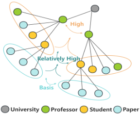
At present, some researches have been devoted to solving the homophily limitation of GNNs. These methods can be mainly divided into two types [Zheng et al., 2022]. 1) Expanding the neighborhood aggregation range and capturing potentially relevant nodes of the anchor node, such as H2GCN [Zhu et al., 2020] and UGCN [Wang et al., 2020]. These works expand the neighborhood range by aggregating multi-hop neighborhoods. Other studies [Wang et al., 2022a; He et al., 2022] typically construct a matrix that expands the neighborhood to the global graph to capture more potentially relevant nodes. 2) Refining the architecture of GNNs, including adaptive message aggregation and inter-layer representation combination. Adaptive message aggregation [Bo et al., 2021; Zhu et al., 2021] is to assign different weights of neighbor nodes during the aggregation process. Inter-layer representation combination [Zhu et al., 2020; Chien et al., 2021] exploits different neighbor ranges by combining intermediate representations of each layer.
These existing methods alleviate the homophily assumption of GNNs to some extent, but they ignore the difference between global information and local information in the aggregation process of GNNs. This causes the aggregation in GNNs fail to provide optimal weights to all potentially relevant nodes, leading to information loss during the aggregation process. For example, MixHop [Abu-El-Haija et al., 2019] and H2GCN [Zhu et al., 2020] consider 2-hop neighbors to aggregate local information. HOG-GCN [Wang et al., 2022a] and BM-GCN [He et al., 2022] consider all neighbors to aggregate global information. However, for local information, the weight distribution of each neighbor node is more easily affected by the local graph topology, resulting in the limited aggregation of local information. For global information, the weight distribution of each neighbor node is more easily affected by the entire graph topology. Therefore, it is important to address the differences between local and global information in the aggregation process of GNNs.
So an intriguing yet important question is how to model the local and global information within graph by making full use of topology and features. Considering the limited information contained in local topology, we innovatively introduce feature similarity to filter out irrelevant nodes. Meanwhile, considering the structural similarity between distant nodes [Jeh and Widom, 2002], we propose a topology-based iterative strategy to capture the global information. Taking an academic graph (shown in Figure 1) as an example, we can find that two professors from the same university are likely to belong to the same labels as they have similar neighborhood topology, such as the students they teach. Moreover, the other two students may also belong to the same labels as they have similar neighborhood topology, such as the papers they published. Not only that, the similarity is transitive, which propagates recursively upward from the low-level similarity topology, and finally infers the high-level professors belong to the same labels. These further illustrates that the node similarity can be inferred through structural similarity.
On the basis of the above-mentioned, we propose a localglobal adaptive graph neural network, namely LG-GNN, for modeling both homophily and heterophily. Specifically, in local modeling, neighbors are divided into high-correlated node sets and low-correlated node sets based on cosine similarity. Then, we use the cosine similarity of the neighbor set of anchor node to generate a sorting matrix, and continuously optimize the sorting matrix during the aggregation process. In global modeling, we introduce SimRank to calculate the structural similarity between node pairs and capture the global information of the anchor node by discovering node pairs with high structural similarity. Finally, we capture the relevant information of the anchor node from both global and local perspectives. Extensive experiments across a series of benchmark datasets illustrate the superiority of LG-GNN over state-of-the-art methods.
2 Preliminaries
We first present the notations, and then give the definition of homophily ratio.
2.1 Notations
Let G = (V,E,X) represent an undirected and unweighted graph, where V = {v1, v2, . . . , vn} represents the node set composed of n nodes, E is the set of edges, X ∈ Rn×f represents the node feature matrix, f represents the dimension of the node features, and each node vi corresponds a feature vector xi in the i-th row of matrix X. The adjacency matrix A = [aij] ∈ Rn×n represents the topology of graph G. If there is an edge between node vi and node vj, aij = 1, otherwise aij = 0.
The proposed model is mainly used in semi-supervised node classification task. In this task, each node has its own label c ∈ C, where |C| represents the number of total classes, and only a few nodes VL ≪ n are associated with corresponding labels. Each node vi ∈ VL has its own one-hot label vector yi ∈ Y = {1, 2, . . . , C}. The goal of semi-supervised node classification is to predict the labels of the remaining nodes V \VL.
2.2 Homophily Ratio
The node-level homophily ratio [Pei et al., 2020] mainly measures the consistency of feature or connection patterns of nodes in the graph. It first calculates the ratio of neighbors of the anchor node with the same label, and then calculates the average ratio of all nodes in the graph, defined as:
where N(vi) is the neighbor set of node vi.
The edge homophily ratio [Zhu et al., 2020] measures the consistency of structure or connection patterns of edges in a graph, which helps to understand the topology and features of the graph. Edge homophily ratio is the ratio of two nodes of the same class connected by one edge, defined as:
3 Methodology
We start with a brief overview and then give the details of each component.
3.1 Overview
In order to tackle the differences between global and local information in the aggregation process, we propose a localglobal adaptive graph neural network, namely LG-GNN, for modeling homophilic and heterophilic graphs. The whole structure of our proposed LG-GNN is displayed in Figure 2.
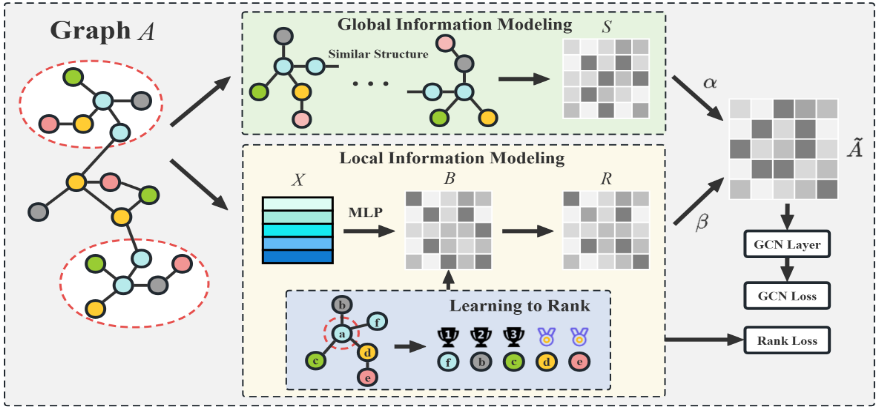
Unlike other GNN models, we use different ways to aggregate global and local information. Specifically, we first integrate the global information based on graph topology similarity and the local information based on learning to rank into adaptive graph convolutional, and then add residual connections to obtain the final node representation. In this way, our method can explore nodes with high similarity to the anchor node globally, and assign ranking scores to neighbors locally. It is worth noting that in the process of adaptive graph convolutional, we model the homophily and heterophily of graph topology, and further update the ranking in local information modeling. Based on these, the neighborhood aggregation can be considered from both topological and feature perspectives.
3.2 Global InformationModeling
In heterophilic graphs, nodes connected to each other often have different labels, while nodes of the same labels are often very far with a long-range dependency relationship. The neighborhood differences of anchor node make it difficult for traditional GNN models to aggregate information from their neighbors, but long-range dependency relationship based on the anchor node is very meaningful for prediction tasks such as node classification. Considering this, we introduce a matrix S to capture long-range dependency information based on the global topology [Jeh and Widom, 2002]. Intuitively, it is believed that if two nodes have similar topology or neighborhoods, two nodes are similar. Therefore, given two nodes vi and vj , the structural similarity between them can be iteratively calculated as:
where c ∈ (0, 1) is the attenuation factor, usually set to 0.6. The higher S(vi, vj), the higher structural similarity. In this way, we can calculate the structural similarity of nodes from an intuitive perspective. Considering that the structural similarity matrix S is defined for any node pair in the graph and is judged by calculating global structural similarity information. Therefore, for the problem of how to discover potentially relevant nodes of anchor node in heterophilic graphs, the structural similarity matrix S can be utilized to assign higher weights to potentially relevant nodes.
In the following, we further analyze the correlation between matrix S and the aggregation process of GNNs from a theoretical perspective. First, we take a look at the concept of random walk [Perozzi et al., 2014]. Random walk refers to starting from a node vi, and selects its neighbor nodes as the next node to move based on a certain probability distribution. This process will continue for multiple steps until the pre-defined number of steps is reached or the pre-defined conditions are reached. Specifically, we use p(vi) = p(vm|vi, r(l) vi:vm ) to represent the probability from node vi to node vm at the pre-defined rule condition r(l) v:m, where vi : vm represents {vi, . . . , vm}. That is, a path of length l consisting of all nodes passing through the path from node vi to node vm. Meanwhile, due to the random nature of the walking process, the anchor nodes' neighbors are visited with equal probability, thus p(vm|vi, r(l) vi:vm ) can be simplified as ∏µ∈rvi:vm 1 |N(µvt )| , where µvt is t-th node on the path r(l) vi:vm . Therefore, the higher value of probability p, the higher the probability of this path. This means that there is a closer connection or association between two nodes, reflecting an increase in similarity or correlation between nodes. Furthermore, according to the properties of Markov chain [Savage, 1972], the steady-state distribution of randomwalks (i.e., the probability of nodes being visited after a long time step) is related to the similarity between nodes. If two nodes have more connections or are more closely related, then the probability of the two nodes being visited during a random walk will be higher, reflecting their similarity.
For traditional GNNs' aggregation, it can be considered as a local random walk with a finite number of steps [Gasteiger et al., 2019], while a random walk with two random nodes can be considered as a global calculation question. The higher the probability of walking between two nodes, the higher the similarity between the two nodes can be inferred. Formally, given two nodes vi and vj, the probability of global random walk can be represented as:
Meanwhile, considering that each layer of most GNN models is propagated and aggregated through the 1-hop neighbors of the anchor node, this process can be regarded as random walk. Therefore, the visit probability of each node can be viewed as a node representation, and the combination of random walk and the node representation learned by GNNs can be represented as z(l) vi [j] = p(vj|vi, r(l) vi:vj ). This indicates that the l layer GNNs can be simulated as a random walk with length l, where the learned node representation contains information about the reachability of multiple nodes on the path. Furthermore, this node representation can be applied to GNNs to simulate a scenario of multi-layer stacking of GNNs, thereby realizing the global random walk of any two nodes. That is, when l →∞, the model is stacked with infinite layers, which is represented as G(∞) . In this way, we can obtain the representations of node vi and node vj in an infinite number of layers, represented as z(l) vi and z(l) vj . Finally, by substituting them into Eq. 3, the structural similarity matrix with global information can be calculated as:
The higher S(vi, vj), the higher weight to nodes vi and vj. By this means, the model can discover potential related nodes of the anchor node in global relationship, and effectively utilize the topology of graph to guide the process of information propagation and aggregation.
3.3 Local InformationModeling
We mainly adopt the method of ListNet loss [Cao et al., 2007] to model local information. The local information matrix aims to predict the ranking of other nodes based on the anchor node and its cosine similarity, and iteratively update the neighbor node ranking of the anchor node during the process of information propagation and aggregation. Specifically, we first use a multi-layer perceptron (MLP) to reduce the dimensionality of node feature matrix X, and obtain the node representation matrix B.
Then, we optimize B by minimizing the cross entropy between the true ranking of nodes in the ranking list and the predicted ranking, and accordlying calculate the local information matrix. Formally, for each neighbor node, we assign a higher ranking to intra-class nodes with high cosine similarity, and assign a lower ranking to inter-class nodes with low cosine similarity. For each given anchor node, there is a corresponding ranking list, as shown in the bottom of Figure 2, and the correct ranking list is predicted by optimizing the loss function. Specifically, for a given anchor node vi, we need to construct a sorting list, which sorts the intra-class nodes and inter-class nodes in the training set based on cosine similarity. The intra-class node ranking list is defined as:
where 1 ≤ qi ≤ Qi, Qi is the number of intra-class nodes in the same labels as node vi, and cos(·) is the cosine similarity. Analogously, the inter-class node ranking list is defined as:
where 1 ≤ qo ≤ Qo, Qo is the number of inter-class nodes in different labels from node vi.
After obtaining the intra-class node ranking list and interclass node ranking list of the anchor node, we combine them into a set of neighbor nodes List(i) = listin i [1 : K]||listout i [-K : -1], where || represents the splicing operation, and the ranking of each node represents its true ranking. This represents the k most similar intra-class nodes and the k least similar inter-class nodes to the anchor node vi in the training set. It is worth noting that in the process of learning to rank, the matrix B is continuously optimized, and the final local information matrix is calculated by R = B · BT .
3.4 Adaptive Graph Convolutional
The above two matrices collect more useful information for the anchor node from both global and local perspectives, allowing for the change of neighborhood propagation weights during the propagation process. In other words, our goal is to increase the influence between intra-class nodes and reduce the influence between inter-class nodes. This means that our global and local information matrices can assign different weights to the neighborhood of the anchor node and capture long-range dependencies under long connections. That is, we can integrate homophily and heterophily. In addition, we separate self-representation from neighborhood representation to preserve more personalized information. Formally, the feature propagation process in the l-th layer can be defined as:
where µ and 1-µ represent the weights of self-representation and neighborhood representation, W (l) n and W (l) e are learnable parameters specific to the l-th layer, α, β and γ represent the weights of local information matrix, global information matrix, and initial matrix, respectively. Z (0) = X is the node feature matrix, and σ is a nonlinear activation function.
The adaptive graph convolutional not only utilizes node features but also utilizes graph topology. For the final result, our approach appears in the form of adding several non-existent edges to a distant set of similar nodes, and deleting several existing edges from a set of dissimilar nodes in the nearby neighborhood (1-hop).
3.5 Optimization Objective
We focus on semi-supervised node classification task, and the loss function of LG-GNN is mainly consists of two parts: Lrank is the loss of learning to rank in local information modeling, and LGCN is the loss of adaptive graph convolutional. Specifically, LG-GNN integrates the global and local information modeling into a unified model. By incorporating the loss functions in local information modeling and in adaptive graph convolutional, the final loss function can be written as:
where softmax is the classification function, |Vtrain| is the number of nodes in the training set, yvi represents true value of vi, and ˆ yvi is the predicted value obtained from the ranking list List(i), which is calculated using Z[i]T · Z[List(i)], representing the product of node vi and relevant node feature information in the ranking list, f(·) is the cross entropy.
4 Experiments
We first introduce the experimental setup, and then evaluate the new approach LG-GNN on node classification and visualization tasks. We finally give a deep investigation on different components of LG-GNN and parameter analysis.
| Datasets | Cora | Cite. | Pubm. | Texa. | Wisc. | Corn. | Film |
|---|---|---|---|---|---|---|---|
| #Nodes | 2,708 | 3,327 | 19,717 | 183 | 251 | 183 | 7,600 |
| #Edges | 5,429 | 4,732 | 44,338 | 309 | 499 | 295 | 33,544 |
| #Features | 1,433 | 3,703 | 500 | 1,703 | 1,703 | 1,703 | 931 |
| #Classes | 7 | 6 | 3 | 5 | 5 | 5 | 5 |
| Hnode | 0.83 | 0.71 | 0.79 | 0.09 | 0.17 | 0.12 | 0.22 |
| Hedge | 0.81 | 0.74 | 0.83 | 0.11 | 0.21 | 0.13 | 0.22 |
4.1 Experimental Setup
Datasets. To demonstrate the performance of LG-GNN in homophilic and heterophilic graphs, we conduct experiments on seven widely used datasets. The statistics of datasets are shown in Table 1.
- Cora, Citeseer, and Pubmed [Sen et al., 2008] are homophilic citation datasets. Among them, nodes represent papers, edges represent citations between papers, node features represent the bag-of-words of the paper, and node labels represent academic topics.
- Texas, Wisconsin, Cornell [Pei et al., 2020], and Film [Tang et al., 2009] are heterophilic datasets. In the first three datasets, nodes represent web pages, edges represent hyperlinks between web pages, node features represent bag-of-words of web pages, and node labels represent page categories. Film is a dataset related to the film industry, where nodes represent actors and edges represent the co-occurrence relationship between two actors on Wikipedia. Node features represent the corresponding keywords for actors in Wikipedia, and labels represent the types of actors identified inWikipedia.
Baselines. We compare our proposed LG-GNN with nine existing methods. They include: 1) Multi-Layer Perceptron (MLP), which only uses node features; 2) Traditional GNN models, including GCN [Kipf and Welling, 2017] and GAT [Veliˇckovi´c et al., 2018], which work under the assumption of homophily; 3) Heterophilic GNN models, including H2GCN [Zhu et al., 2020], GOAL [Zheng et al., 2023], SIMGA [Liu et al., 2023], HOG-GCN [Wang et al., 2022a], BM-GCN [He et al., 2022], and OrderedGNN [Song et al., 2023].
Implementation Details. The experiment generated 10 random partitions on the datasets. For each dataset, 48% of nodes are used to training set, 32% of nodes are used to validation set, and the remaining 20% are used to test set. For fair comparison, all methods use the same 10 random partitions. In addition, for all baselines, we adopt the default parameters used by the authors in the original paper. For our LG-GNN, a two-layer MLP is used in the local information modeling to process the feature matrix X, with the dimension of 512 of hidden layer. In the process of adaptive graph convolutional, a two-layer graph convolutional operation is used, and the dimension of hidden layer is 256. For hyperparameters, we use the weight of the local information matrix with α = 0.2, the weight of the global information matrix with β = 0.4, the initial matrix weight with β = 1, the self-representation weight with µ = 0.5, and the learning rate to 0.001.
4.2 Node Classification
The results of node classification are shown in Table 2, with the average accuracy and standard deviation of 10 random partitions as evaluation indicators. As shown, we can find that LG-GNN performs best in 5 out of 7 datasets and still maintains a competitive level in the remaining two datasets. The detailed analysis is as follows:
- Our LG-GNN maintains optimal performance or strong competitiveness on homophilic datasets (i.e., Cora, Citeseer, and Pubmed). Specifically, LG-GNN performs the best on Cora and Pumbed, with a 0.15% difference from the best performing OrderedGNN on Citeseer, still maintaining a competitive level. The experimental results indicate that our method has the best or highly competitive performance on homophilic datasets.
- LG-GNN performs the best on four heterophilic datasets, namely Texas, Wisconsin, Cornell, and Film. Specifically, LG-GNN is superior to traditional GNN models, with an average improvement of 28.50% and 26.50% compared to GCN and GAT, and an average improvement of 3.70% compared to MLP that only
| Methods | Cora | Citeseer | Pubmed | Texas | Wisconsin | Cornell | Film |
|---|---|---|---|---|---|---|---|
| MLP | 71.29±1.60 | 66.96±2.61 | 86.48±0.63 | 81.08±4.83 | 85.49±3.53 | 83.24±7.03 | 36.58±1.44 |
| GCN | 86.48±1.43 | 72.67±1.99 | 87.34±0.65 | 54.05±4.36 | 50.39±7.55 | 53.78±8.59 | 28.78±1.48 |
| GAT | 87.16±1.17 | 75.64±1.95 | 85.25±0.60 | 57.30±3.38 | 54.31±5.62 | 54.59±7.33 | 28.99±1.44 |
| H2GCN | 86.48±1.63 | 75.56±2.18 | 88.77±0.65 | 79.73±7.27 | 82.55±4.33 | 78.38±4.35 | 36.71±1.41 |
| GOAL | 88.71±0.87 | 77.15±0.95 | 89.25±0.55 | 85.92±4.28 | 87.15±3.71 | 85.46±4.52 | 36.74±1.41 |
| SIMGA | 88.41±1.33 | 77.22±1.52 | 89.56±0.31 | 84.87±4.39 | 87.92±3.64 | 85.76±4.49 | 36.81±1.21 |
| HOG-GCN | 85.17±4.40 | 76.15±1.88 | 88.79±0.40 | 85.17±4.40 | 86.67±3.36 | 84.32±4.32 | 36.82±0.84 |
| BM-GCN | 87.99±1.29 | 76.13±1.92 | 90.25±0.75 | 85.13±4.64 | 86.87±3.42 | 84.74±4.41 | 36.46±1.24 |
| OrderedGNN | 88.37±0.75 | 77.31±1.73 | 90.15±0.38 | 86.22±4.12 | 88.04±3.63 | 86.35±4.73 | 36.91±1.46 |
| LG-GNN | 88.73±1.24 | 77.16±1.89 | 89.76±0.67 | 89.20±2.29 | 88.24±3.49 | 86.49±4.84 | 37.24±0.91 |
uses features. For traditional GNN models, the drawback of only being able to aggregate the mean on heterophilic graphs is significantly magnified, resulting in a decrease in model accuracy. Compared with other GNN models specifically designed for heterophilic datasets (i.e., H2GCN, GOAL, SIMGA, HOG-GCN, BM-GCN, and OrderedGNN), the average accuracy of LG-GNN has improved by 0.97%-5.90%. These results further demonstrate the effectiveness and superiority of integrating both local and global information adaptively for modeling heterophily.
4.3 Visualization
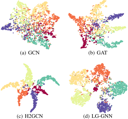
In order to analyze the effectiveness of node representation learned by LG-GNN more intuitively, we visualize node embeddings on the CiteSeer dataset using t-SNE [Van der Maaten and Hinton, 2008]. The visualization results of GCN, GAT, H2GCN, and LG-GNN are shown in Figure 3, where different colors represent nodes with different labels. An ideal visualization result is that nodes of the same classes (in the same color) should be close to each other.
As shown, the visualization results of GCN and GAT are relatively poor, where nodes with different labels are mixed together, indicating poor clustering performance. Compared to H2GCN, our proposed LG-GNN has a more clear class boundary, so the visualization effect of LG-GNN is better than H2GCN. This is also consistent with the node classification results, which indirectly verifies the effectiveness of our local-global adaptive graph neural network for modeling both homophily and heterophily.
4.4 Ablation Study
To verify the effectiveness of each component of LG-GNN, we conduct experiments on comparing LG-GNN with four variations. The variants are as follows: 1) GCN, which serves as the base framework of LG-GNN; 2) LG-GNN-1: removing the global information modeling of LG-GNN; 3) LG-GNN2: removing the local information modeling; 4) LG-GNN-3: removing residual connections.
As shown in Table 3, all three variants have higher average accuracy than GCN on seven datasets and lower accuracy than LG-GNN, indicating that using both local and global information can significantly improve the node classification results of the model on homophilic and heterophilic graphs. In addition, the average performance of LG-GNN-1 is better than that of LG-GNN-2, indicating better improvement in local information modeling.
| Methods | Cora | Citeseer | Pubmed | Texas | Wisconsin | Cornell | Film |
|---|---|---|---|---|---|---|---|
| GCN | 86.48 | 72.67 | 87.34 | 54.05 | 50.39 | 53.78 | 28.78 |
| LG-GNN-1 | 87.32 | 73.35 | 87.96 | 81.92 | 78.43 | 86.49 | 34.81 |
| LG-GNN-2 | 81.49 | 73.58 | 85.71 | 83.78 | 80.39 | 83.78 | 33.51 |
| LG-GNN-3 | 88.23 | 76.14 | 89.12 | 88.30 | 86.12 | 85.12 | 35.87 |
| LG-GNN | 88.73 | 77.16 | 89.76 | 89.20 | 88.24 | 86.49 | 37.24 |
4.5 Parameter Analysis
We take homophilic dataset Cora and heterophilic dataset Texas as examples to analyze the sensitivity of hyperparameters of LG-GNN.
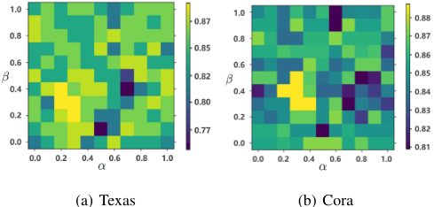
Analysis of weight α and β. The parameters α and β represent the weights of the local information matrix and the global information matrix, respectively. We vary their value from 0 to 1, and the corresponding results are shown in Figure 4. On the heterophilic dataset Texas, when α and β are 0, (i.e., only the global information matrix or only the local information matrix is used), the performance is relatively poor. When α and β are in the range of 0.2 to 0.4, LG-GNN has the best model performance. On the homophilic dataset Cora, when α and β are 0, the performance is relatively poor. When α and β are in the range of 0.2 to 0.4, our LG-GNN has the highest performance. In summary, the model performs best with parameters α = 0.2 and β = 0.4 on both heterophilic and homophilic datasets.
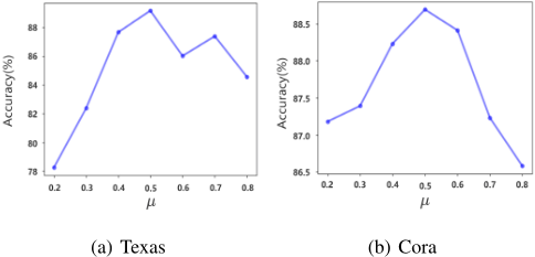
Analysis of weight µ. The parameter µ represents the weight of the proportion of self-representation and neighborhood representation. The corresponding results are shown in Figure 5. It can be find that as µ first increases and then decreases, the maximum accuracy is obtained when µ = 0.5. In particular, µ = 0 means that only self-representation is used for convolution, while µ = 1 means that only neighborhood representation is used for convolution. In both cases, the performance of the model is at its best. When in a mixed state using self-representation and neighborhood representation, the model performance is significantly improved, and the model performance is best when µ = 0.5.
5 RelatedWork
According to the focus of this paper, we briefly review related research on classical graph neural networks and heterophilic graph neural networks.
Classical Graph Neural Networks. GCN [Kipf and Welling, 2017] introduces traditional convolutional operations into graph neural networks and uses the features of neighbor nodes to update the node representations. In order to solve the equality problem of GCN for neighbor nodes when aggregating information, GAT [Veliˇckovi´c et al., 2018] introduces an attention mechanism to learn the importance scores between each node and its neighbor nodes, and then aggregates neighbor information based on these scores. Further, GraphSAGE [Hamilton et al., 2017] samples the neighbors of each node at each layer, and uses aggregation functions (such as mean, maximum, etc.) to aggregate the sampled neighbor information, which has good scalability and efficiency, especially suitable for large-scale graph data.
Heterophilic Graph Neural Networks. To overcome the limitations of homophily assumption of GNNs, H2GCN [Zhu et al., 2020] proposes three key designs: self-neighbor separation, high-order neighborhood, and intermediate combination to capture information at low levels of homophily. Geom-GCN [Pei et al., 2020] defines a new geometric relationship by adding neighborhoods that comply with the defined geometric relationship to the message aggregation of GCN. HOG-GCN [Wang et al., 2022a] calculates the probability of a pair of nodes belonging to the same class by constructing a same attitude matrix. After that, BM-GCN [He et al., 2022] adopts different rules for aggregation of intra- and inter-class nodes by constructing a block similarity matrix. OrderedGNN [Song et al., 2023] alleviates the assumption of homophily by sorting the nodes in the graph and strictly following the node order during the process of information propagation and aggregation.
These existing methods have achieved great results in handling the homophily assumption of GNNs. However, existing GNN methods often overlook the differences between global and local patterns, which is very important for information propagation and aggregation.
6 Conclusion
This paper proposes a graph neural network that adaptively integrates global and local information, so as to handle both homophilic and heterophilic graphs simultaneously. The model explores the potentially relevant nodes of the target from a global perspective using structural similarity and learns local ordering through feature similarity. These two components are then integrated into the adaptive graph convolutional to address the differences between global and local information during the aggregation process. Experiments on seven real-world datasets demonstrate that our proposed LGGNN outperforms existing methods on heterophilic graphs and remains competitive on homophilic graphs.
Acknowledgments
This work is supported by National Key Research and Development Program of China (2023YFC3304503, 2023YFB2603904), National Natural Science Foundation of China (62276187).
@inproceedings{ijcai2024p278,
  title     = {LG-GNN: Local-Global Adaptive Graph Neural Network for Modeling Both Homophily and Heterophily},
  author    = {Yu, Zhizhi and Feng, Bin and He, Dongxiao and Wang, Zizhen and Huang, Yuxiao and Feng, Zhiyong},
  booktitle = {Proceedings of the Thirty-Third International Joint Conference on
               Artificial Intelligence, {IJCAI-24}},
  publisher = {International Joint Conferences on Artificial Intelligence Organization},
  editor    = {Kate Larson},
  pages     = {2515--2523},
  year      = {2024},
  month     = {8},
  note      = {Main Track},
  doi       = {10.24963/ijcai.2024/278},
  url       = {https://doi.org/10.24963/ijcai.2024/278},
}
TY - CPAPER TI - LG-GNN: Local-Global Adaptive Graph Neural Network for Modeling Both Homophily and Heterophily AU - Yu, Zhizhi AU - Feng, Bin AU - He, Dongxiao AU - Wang, Zizhen AU - Huang, Yuxiao AU - Feng, Zhiyong T2 - Proceedings of the Thirty-Third International Joint Conference on Artificial Intelligence, IJCAI-24 PB - International Joint Conferences on Artificial Intelligence Organization PY - 2024 SP - 2515 EP - 2523 DO - 10.24963/ijcai.2024/278 UR - https://doi.org/10.24963/ijcai.2024/278 ER -Copied
Machine-readable versions of this paper, for tools and AI agents:





