
Sub-Adjacent Transformer: Improving Time Series Anomaly Detection with Reconstruction Error from Sub-Adjacent Neighborhoods
Proceedings of the Thirty-Third International Joint Conference on Artificial Intelligence. Main Track. Pages 2524-2532.
https://doi.org/10.24963/ijcai.2024/279
Keywords
- Machine Learning: ML: Time series and data streams
- Data Mining: DM: Anomaly/outlier detection
Abstract
In this paper, we present the Sub-Adjacent Transformer with a novel attention mechanism for unsupervised time series anomaly detection. Unlike previous approaches that rely on all the points within some neighborhood for time point reconstruction, our method restricts the attention to regions not immediately adjacent to the target points, termed sub-adjacent neighborhoods. Our key observation is that owing to the rarity of anomalies, they typically exhibit more pronounced differences from their sub-adjacent neighborhoods than from their immediate vicinities. By focusing the attention on the sub-adjacent areas, we make the reconstruction of anomalies more challenging, thereby enhancing their detectability. Technically, our approach concentrates attention on the non-diagonal areas of the attention matrix by enlarging the corresponding elements in the training stage. To facilitate the implementation of the desired attention matrix pattern, we adopt linear attention because of its flexibility and adaptability. Moreover, a learnable mapping function is proposed to improve the performance of linear attention. Empirically, the Sub-Adjacent Transformer achieves state-of-the-art performance across six real-world anomaly detection benchmarks, covering diverse fields such as server monitoring, space exploration, and water treatment.
- [Abdulaal et al., 2021] Ahmed Abdulaal, Zhuanghua Liu, and Tomer Lancewicki. Practical approach to asyn- chronous multivariate time series anomaly detection and localization. In SIGKDD, pages 2485-2494, 2021.
- [Ahmed et al., 2017] Chuadhry Mujeeb Ahmed, Venkata Reddy Palleti, and Aditya P. Mathur. Wadi: a water distribution testbed for research in the design of secure cyber physical systems. In Proceedings of the 3rd international workshop on cyber-physical systems for smart water networks, pages 25-28, 2017.
- [Audibert et al., 2020] Julien Audibert, Pietro Michiardi, Frédéric Guyard, Sébastien Marti, and Maria A. Zuluaga. Usad: Unsupervised anomaly detection on multivariate time series. In SIGKDD, pages 3395-3404, 2020.
- [Blázquez-García et al., 2021] Ane Blázquez-García, Angel Conde, Usue Mori, and Jose A Lozano. A review on out- lier/anomaly detection in time series data. ACM Comput- ing Surveys, 54(3):1-33, April 2021.
- [Bolya et al., 2022] Daniel Bolya, Cheng-Yang Fu, Xiao- liang Dai, Peizhao Zhang, and Judy Hoffman. Hydra at- tention: Efficient attention with many heads. In ECCV, pages 35-49. Springer, 2022.
- [Boniol and Palpanas, 2022] Paul Boniol and Themis Palpanas. Series2graph: Graph-based subsequence anomaly detection for time series. arXiv preprint arXiv:2207.12208, 2022.
- [Breunig et al., 2000] Markus M Breunig, Hans-Peter Kriegel, Raymond T. Ng, and Jörg Sander. Lof: iden- tifying density-based local outliers. In SIGMOD, pages 93-104, 2000.
- [Brown et al., 2020] Tom Brown, Benjamin Mann, Nick Ry- der, Melanie Subbiah, Jared D Kaplan, Prafulla Dhari- wal, Arvind Neelakantan, Pranav Shyam, Girish Sastry, Amanda Askell, et al. Language models are few-shot learners. NIPS, 33:1877-1901, 2020.
- [Cai et al., 2023] Han Cai, Chuang Gan, and Song Han. Efficientvit: Lightweight multi-scale attention for high- resolution dense prediction. In ICCV, pages 17302-17313, 2023.
- [Chen et al., 2021] Zekai Chen, Dingshuo Chen, Xiao Zhang, Zixuan Yuan, and Xiuzhen Cheng. Learning graph structures with transformer for multivariate time-series anomaly detection in iot. IEEE Internet of Things Jour- nal, 9(12):9179-9189, 2021.
- [Chen, 2018] Tiankai Chen. Anomaly detection in semicon- ductor manufacturing through time series forecasting us- ing neural networks. PhD thesis, Massachusetts Institute of Technology, 2018.
- [Cheng et al., 2008] Haibin Cheng, Pang-Ning Tan, Christo- pher Potter, and Steven Klooster. A robust graph-based al- gorithm for detection and characterization of anomalies in noisy multivariate time series. In ICDM workshops, pages 349-358. IEEE, 2008.
- [Deng and Hooi, 2021] Ailin Deng and Bryan Hooi. Graph neural network-based anomaly detection in multivariate time series. In AAAI, volume 35, pages 4027-4035, 2021.
- [Ding et al., 2019] Nan Ding, HaoXuan Ma, Huanbo Gao, YanHua Ma, and GuoZhen Tan. Real-time anomaly de- tection based on long short-term memory and gaussian mixture model. Computers & Electrical Engineering, 79:106458, 2019.
- [Fox, 1972] Anthony J Fox. Outliers in time series. Jour- nal of the Royal Statistical Society Series B: Statistical Methodology, 34(3):350-363, 1972.
- [Garg et al., 2022] Astha Garg, Wenyu Zhang, Jules Sama- ran, Ramasamy Savitha, and Chuan-Sheng Foo. An eval- uation of anomaly detection and diagnosis in multivariate time series. IEEE Transactions on Neural Networks and Learning Systems, 33(6):2508-2517, 2022.
- [Gupta et al., 2013] Manish Gupta, Jing Gao, Charu C. Ag- garwal, and Jiawei Han. Outlier detection for temporal data: A survey. IEEE Transactions on Knowledge and data Engineering, 26(9):2250-2267, 2013.
- [Han et al., 2023] Dongchen Han, Xuran Pan, Yizeng Han, Shiji Song, and Gao Huang. Flatten transformer: Vision transformer using focused linear attention. In ICCV, pages 5961-5971, 2023.
- [Ho et al., 2020] Jonathan Ho, Ajay Jain, and Pieter Abbeel. Denoising diffusion probabilistic models. NIPS, 33:6840- 6851, 2020.
- [Hundman et al., 2018a] Kyle Hundman, Valentino Con- stantinou, Christopher Laporte, Ian Colwell, and Tom Soderstrom. Detecting spacecraft anomalies using lstms and nonparametric dynamic thresholding. In SIGKDD, pages 387-395, 2018.
- [Hundman et al., 2018b] Kyle Hundman, Valentino Con- stantinou, Christopher Laporte, Ian Colwell, and Tom Soderstrom. Detecting spacecraft anomalies using lstms and nonparametric dynamic thresholding. In SIGKDD, pages 387-395, 2018.
- [Katharopoulos et al., 2020] Angelos Katharopoulos, Apoorv Vyas, Nikolaos Pappas, and Franc ¸ois Fleuret. Transformers are rnns: Fast autoregressive transformers with linear attention. In ICML, pages 5156-5165. PMLR, 2020.
- [Kieu et al., 2019] Tung Kieu, Bin Yang, Chenjuan Guo, and Christian S. Jensen. Outlier detection for time series with recurrent autoencoder ensembles. In IJCAI, pages 2725- 2732, 2019. IJCAI
- [Kingma and Ba, 2015] Diederik P. Kingma and Jimmy Ba. Adam: A method for stochastic optimization. In ICLR, 2015.
- [Lai et al., 2021] Kwei-Herng Lai, Daochen Zha, Junjie Xu, Yue Zhao, Guanchu Wang, and Xia Hu. Revisiting time series outlier detection: Definitions and benchmarks. In NeurIPS Dataset and Benchmark Track, 2021.
- [Lai et al., 2023] Chih-Yu Lai, Fan-Keng Sun, Zhengqi Gao, Jeffrey H Lang, and Duane S Boning. Nom- inality score conditioned time series anomaly detec- tion by point/sequential reconstruction. arXiv preprint arXiv:2310.15416, 2023.
- [Li et al., 2019] Dan Li, Dacheng Chen, Baihong Jin, Lei Shi, Jonathan Goh, and See-Kiong Ng. Mad-gan: Multi- variate anomaly detection for time series data with gener- ative adversarial networks. In International conference on artificial neural networks, pages 703-716. Springer, 2019.
- [Li et al., 2021] Zhihan Li, Youjian Zhao, Jiaqi Han, Ya Su, Rui Jiao, Xidao Wen, and Dan Pei. Multivariate time se- ries anomaly detection and interpretation using hierarchi- cal inter-metric and temporal embedding. In SIGKDD, pages 3220-3230, 2021.
- [Liu et al., 2013] Bo Liu, Yanshan Xiao, Longbing Cao, Zhifeng Hao, and Feiqi Deng. Svdd-based outlier detec- tion on uncertain data. Knowledge and information sys- tems, 34:597-618, 2013.
- [Liu et al., 2021] Ze Liu, Yutong Lin, Yue Cao, Han Hu, Yixuan Wei, Zheng Zhang, Stephen Ching-Feng Lin, and Baining Guo. Swin transformer: Hierarchical vision trans- former using shifted windows. In ICCV, pages 10012- 10022, 2021.
- [Mathur and Tippenhauer, 2016] Aditya P. Mathur and Nils Ole Tippenhauer. Swat: a water treatment testbed for research and training on ics security. In CySWATER, pages 31-36. IEEE, 2016.
- [Park et al., 2018] Daehyung Park, Yuuna Hoshi, and Charles C Kemp. A multimodal anomaly detector for robot-assisted feeding using an lstm-based variational autoencoder. IEEE Robotics and Automation Letters, 3(3):1544-1551, 2018.
- [Pereira and Silveira, 2019] João Pereira and Margarida Sil- veira. Learning representations from healthcare time series data for unsupervised anomaly detection. In 2019 IEEE international conference on big data and smart computing (BigComp), pages 1-7. IEEE, 2019.
- [Pintilie et al., 2023] Ioana Pintilie, Andrei Manolache, and Florin Brad. Time series anomaly detection using diffusion-based models. arXiv preprint arXiv:2311.01452, 2023.
- [Schmidl et al., 2022] Sebastian Schmidl, Phillip Wenig, and Thorsten Papenbrock. Anomaly detection in time series: a comprehensive evaluation. Proceedings of the VLDB Endowment, 15(9):1779-1797, 2022.
- [Schölkopf et al., 2001] Bernhard Schölkopf, John C. Platt, J. Shawe-Taylor, Alex Smola, and R. C. Williamson. Es- timating the support of a high-dimensional distribution. Neural computation, 13(7):1443-1471, 2001.
- [Shen et al., 2020] Lifeng Shen, Zhuocong Li, and James T. Kwok. Timeseries anomaly detection using temporal hier- archical one-class network. NIPS, 33:13016-13026, 2020.
- [Shen et al., 2021] Zhuoran Shen, Mingyuan Zhang, Haiyu Zhao, Shuai Yi, , and Hongsheng Li. Efficient attention: Attention with linear complexities. In WACV, pages 3531- 3539, 2021.
- [Su et al., 2019] Ya Su, Youjian Zhao, Chenhao Niu, Rong Liu, Wei Sun, and Dan Pei. Robust anomaly detection for multivariate time series through stochastic recurrent neural network. In SIGKDD, pages 2828-2837, 2019.
- [Sun et al., 2021] Fan-Keng Sun, Chris Lang, and Duane Boning. Adjusting for autocorrelated errors in neural net- works for time series. NIPS, 34:29806-29819, 2021.
- [Tax and Duin, 2004] David M.J. Tax and Robert P.W. Duin. Support vector data description. Machine learning, 54:45- 66, 2004.
- [Tuli et al., 2022] Shreshth Tuli, Giuliano Casale, and Nicholas R Jennings. Tranad: Deep transformer net- works for anomaly detection in multivariate time series data. arXiv preprint arXiv:2201.07284, 2022.
- [Vaswani et al., 2017] Ashish Vaswani, Noam Shazeer, Niki Parmar, Jakob Uszkoreit, Llion Jones, Aidan N Gomez, Łukasz Kaiser, and Illia Polosukhin. Attention is all you need. NIPS, 30, 2017.
- [Wu et al., 2023] Haixu Wu, Tengge Hu, Yong Liu, Hang Zhou, Jianmin Wang, and Mingsheng Long. Timesnet: Temporal 2d-variation modeling for general time series analysis. ICLR, 2023.
- [Xu et al., 2022] Jiehui Xu, Haixu Wu, Jianmin Wang, and Mingsheng Long. Anomaly transformer: Time series anomaly detection with association discrepancy. In ICLR, 2022.
- [Zhang et al., 2019] Chuxu Zhang, Dongjin Song, Yuncong Chen, Xinyang Feng, Cristian Lumezanu, Wei Cheng, Jingchao Ni, Bo Zong, Haifeng Chen, and Nitesh V Chawla. A deep neural network for unsupervised anomaly detection and diagnosis in multivariate time series data. In AAAI, volume 33, pages 1409-1416, 2019.
- [Zhao et al., 2020] Hang Zhao, Yujing Wang, Juanyong Duan, Congrui Huang, Defu Cao, Yunhai Tong, Bixiong Xu, Jing Bai, Jie Tong, and Qi Zhang. Multivariate time- series anomaly detection via graph attention network. In ICDM, pages 841-850. IEEE, 2020.
- [Zhao et al., 2022] Yan Zhao, Liwei Deng, Xuanhao Chen, Chenjuan Guo, Bin Yang, Tung Kieu, Feiteng Huang, Tor- ben Bach Pedersen, Kai Zheng, and Christian S Jensen. A comparative study on unsupervised anomaly detection for time series: Experiments and analysis. arXiv preprint arXiv:2209.04635, 2022.
- [Zhou et al., 2019] Bin Zhou, Shenghua Liu, Bryan Hooi, Xueqi Cheng, and Jing Ye. Beatgan: Anomalous rhythm detection using adversarially generated time series. In IJ- CAI, volume 2019, pages 4433-4439, 2019. IJCAI
- [Zong et al., 2018] Bo Zong, Qi Song, Martin Renqiang Min, Wei Cheng, et al. Deep autoencoding gaussian mix- ture model for unsupervised anomaly detection. In ICLR, 2018.
References were extracted automatically from the PDF and may contain errors.
Full text extracted automatically from the PDF; figures, tables and equations may differ. The PDF is the version of record.
1 Introduction
In modern industrial systems such as data centers and smart factories, numerous sensors consistently produce significant volumes of measurements [Zhou et al., 2019; Shen et al., 2020]. To effectively monitor the systems' real-time conditions and avoid potential losses, it is crucial to identify anomalies in the multivariate time series [Pereira and Silveira, 2019; Chen, 2018]. This problem is known as time series anomaly detection [Bl´azquez-Garc´ıa et al., 2021]. Comprehensive surveys can be found in the literature [Bl´azquezGarc´ıa et al., 2021; Schmidl et al., 2022; Gupta et al., 2013].
∗ Corresponding Author
(a) Existing Methods
(b) Our Method
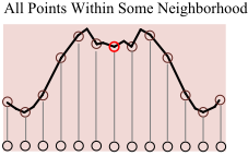
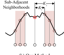
Figure 1: Illustration of our method in time domain. The point marked with a red circle, along with its neighbors, represents an anomaly on the sinusoidal signal. (a) Previous works typically utilize the attention across all the points within the window, while (b) our method encourages the use of attention of sub-adjacent neighborhoods (the highlighted area). Such an imposed constraint enlarges the reconstruction challenge for anomalies and thus improves the anomaly detection performance.
Effective and robust time series anomaly detection remains a challenging and open problem [Zhao et al., 2022]. Realworld time series usually exhibit nonlinear dependencies and intricate interactions among time points. Besides, the vast scale of data makes the labeling of these anomalies timeconsuming and costly in practice [Lai et al., 2023]. Therefore, time series anomaly detection is usually conducted in an unsupervised manner [Xu et al., 2022], which is also the focus of this paper.
Before the era of deep learning, many classic anomaly detection methods were proposed. These include the densityestimation method proposed in [Breunig et al., 2000], the clustering-based method presented in one-class SVM [Sch¨olkopf et al., 2001], and a series of SVDD works [Tax and Duin, 2004; Liu et al., 2013], along with graph-based methods [Cheng et al., 2008]. Traditional methods, which use handcrafted features, struggle to accurately express the relationship among time points and often suffer from poor generalization. Deep learning-based techniques have witnessed a diversity of methods during the recent decade. Broadly, they can be categorized into three main categories: Reconstruction-based methods reconstruct the time series and compare it with the original data [Park et al., 2018;
Li et al., 2021; Su et al., 2019; Pintilie et al., 2023], whereas prediction-based methods predict future points for comparison with actual data [Deng and Hooi, 2021; Hundman et al., 2018a; Ding et al., 2019; Lai et al., 2023]. Dissimilaritybased methods emphasize the discrepancy representation between normal and abnormal points in various domains [Shen et al., 2020; Sun et al., 2021; Xu et al., 2022]. It is noteworthy that these methods often combine multiple approaches to enhance performance. For example, TranAD [Tuli et al., 2022] integrates an integrated reconstruction error and discriminator loss; while [Lai et al., 2023] uses prediction results as the nominal data and combines them with reconstruction results.
In this paper, we focus on the attention matrix within the Transformer module. Transformers [Vaswani et al., 2017] have achieved great success in natural language processing [Brown et al., 2020], computer vision [Liu et al., 2021] and time series [Xu et al., 2022] in recent years. Previous work in [Xu et al., 2022] primarily concentrated on the dissimilarities in attention distributions. Our paper takes a different approach and introduces a simple yet effective attention learning paradigm. Our fundamental assumption is that anomalies are less related to their non-immediate neighborhoods when compared with normal points. Therefore, focusing exclusively on these non-immediate neighborhoods is likely to result in larger reconstruction errors for anomalies. Based on this assumption, our study introduces two key concepts: subadjacent neighborhoods and sub-adjacent attention contribution. As shown in Figure 1, sub-adjacent neighborhoods indicate the areas not immediately adjacent to the target point, and the sub-adjacent attention contribution is defined as the sum of particular non-diagonal elements in the corresponding column of the attention matrix. These concepts are integrated with reconstruction loss, forming the cornerstone of our anomaly detection strategy. Furthermore, we observe that the traditional Softmax operation used in standard selfattention impedes the formation of the desired attention matrix, where the predefined non-diagonal stripes are dominant. In response, we adopt linear attention [Shen et al., 2021; Han et al., 2023] for its greater flexibility in attention matrix configurations. We also tailor the mapping function within this framework, using learnable parameters to enhance performance. The main contributions of this paper are summarized as follows.
- We propose a novel attention learning regime based on the sub-adjacent neighborhoods and attention contribution. Specifically, a new attention matrix pattern is designed to enhance discrimination between anomalies and normal points.
- Furthermore, we leverage the linear attention to achieve the desired attention pattern. To the best of our knowledge, this is the first introduction of linear attention with a learnable mapping function to time series anomaly detection.
- Extensive experiments show that the proposed SubAdjacent Transformer delivers state-of-the-art (SOTA) performance across six real-world benchmarks and one synthetic benchmark.
2 RelatedWorks
Time Series Anomaly detection. In recent year, graph neural networks and self-attention have been explored in time series anomaly detection [Deng and Hooi, 2021; Zhao et al., 2020; Boniol and Palpanas, 2022; Xu et al., 2022; Lai et al., 2023; Wu et al., 2023]. The most related work to ours is Anomaly Transformer [Xu et al., 2022], which also exploits the attention information. The discrepancy between the learned Gaussian distribution and the actual distribution is used to distinguish abnormal points from normal ones. A somewhat complicated min-max training strategy is adopted to train the model. Generally, Anomaly Transformer is complex and somewhat indirect. Our proposed method is more straightforward and exhibits improved performance.
Linear Attention. Compared with vanilla self-attention, linear attention enjoys more flexibility and lighter computation burden. Existing linear attention methods can be divided into three categories: pattern based methods, kernel based methods and mapping based methods. We mainly focus on mapping based methods in this paper. Efficient attention [Shen et al., 2021] applies Softmax function to Q (in a row-wise manner) and 𝐾 (in a column-wise manner) to ensure each row of QK 𝑇 sums up to 1. Hydra attention [Bolya et al., 2022] studies the special case where attention heads are as many as feature dimension and Q and K are normalized so that ∥Q𝑖 ∥ and ∥K𝑖 ∥ share the same value. EfficientVit [Cai et al., 2023] uses the simple ReLU function as the mapping function. FLatten Transformer [Han et al., 2023] proposes the power function as the mapping function to improve the focus capability. In this paper, we apply Softmax to matrices Q and K both in a row-wise manner to approximate the focus property of the vanilla self-attention. Empirical experiments verify its performance superiority to other mapping methods in time series anomaly detection.
3 Methods
3.1 ProblemFormulation
Let X = {x1, · · · , x𝑇} ∈ R 𝑇×𝐷 denote a set of time series with x𝑡 ∈ R 𝐷 , where 𝑇 is the time steps and 𝐷 is the number of channels. The label vector y = {𝑦1, · · · , 𝑦𝑇} indicates whether the corresponding time stamp is normal (𝑦𝑡 = 0) or abnormal (𝑦𝑡 = 1). Our task is to determine anomaly labels for all time points ˆy = { ˆ𝑦1, · · · , ˆ𝑦𝑡 }, where ˆ𝑦𝑡 ∈ {0, 1}, to match the ground truth y as much as possible. Following the practice of [Xu et al., 2022; Schmidl et al., 2022; Tuli et al., 2022; Lai et al., 2023], we mainly focus on the F1 score with point adjustment.
3.2 Sub-Adjacent Neighborhoods
Time points usually have stronger connections with their neighbors and fewer connections with distant points. This characteristic is more pronounced for anomalies [Xu et al., 2022]. As shown in Figure 1, if we rely solely on subadjacent neighborhoods to reconstruct time points, the reconstruction errors of anomalies will become more pronounced, thereby enhancing their distinguishability. This is the core idea of the Sub-Adjacent Transformer.
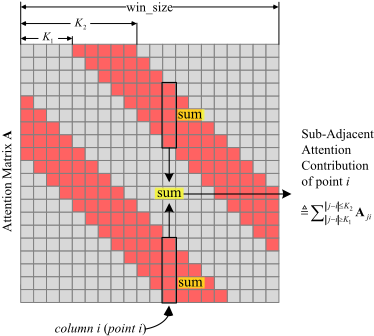
In this paper, we define the sub-adjacent neighborhoods as the region where the distance to the target point is between K1 and K2. 𝐾1 and 𝐾1 are the pre-defined area bounds and satisfy 𝐾2 ≥ 𝐾1 > 0. The highlighted red area in Figure 1 (b) show the sub-adjacent neighborhoods of the point marked with the red circle.
We now apply our thought to the attention matrix. The subadjacent neighborhoods are represented by the highlighted stripes in the attention matrix, as depicted in Figure 2. To focus attention on these stripes, we introduce the concept of attention contribution. This concept involves viewing the columns of the attention matrix as each point's contribution to others within the same window. Let A𝑖 𝑗 denote the element in the 𝑖-th row and 𝑗-th column of the attention matrix A. The value of A𝑖 𝑗 reflects the extent of point 𝑖's contribution to point 𝑗; the larger A𝑖 𝑗 is, the more significant the contribution. We define the sub-adjacent attention contribution of each point as the aggregate of values within the pre-defined sub-adjacent span in the corresponding column, which is
where subscript (:, 𝑖) denotes the 𝑖th column of the corresponding matrix, and win size is the window size.
The sub-adjacent attention contribution plays a pivotal role in two aspects. Firstly, it steers the focus of attention towards the sub-adjacent neighborhoods by being integrated into the loss function (Eq. 5). This is achieved by increasing SACon (A) for all points during the training stage. Secondly, it assists in anomaly detection. This is due to its incorporation into the anomaly score calculation, where anomalies typically show a lower attention contribution than normal points.
Moreover, the number of the highlighted cells in Figure 2 is lower for the marginal points (where 𝑖 < 𝐾2 or 𝑖 > win size𝐾2), leading to imbalance among points. It is mainly because the 𝑗 in Eq. 1 is bounded by 0 ≤ 𝑗 < 𝑤𝑖𝑛 𝑠𝑖𝑧𝑒. To break through this limitation, one plausible way is to use a circular shift function to calculate A𝑗𝑖 in Eq. 1:
where Q,K ∈ R win size×dmodel are the query and key matrix, respectively, ⟨·, ·⟩ represents the inner product of two vectors, Roll (Q, 𝑖 - 𝑗) cyclically shift matrix Q by 𝑖 - 𝑗 along the first dimension. The 𝑗 values in A𝑗𝑖 of Eq. 2 can satisfy the conditions 𝑗 < 0 or 𝑗 ≥ 𝑤𝑖𝑛 𝑠𝑖𝑧𝑒 and ensure that the number of 𝑗s for each 𝑖 is the same. Actually, the cyclic operation in Eq. 2 is equivalent to setting SACon � A:,𝑖 � in Eq. 1 as:
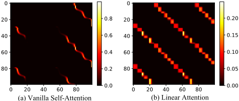
where [ 𝑗] = 𝑗 +𝑛 · 𝑤𝑖𝑛 𝑠𝑖𝑧𝑒, 𝑛 ∈ {0, ±1} such that 0 ≤ [ 𝑗] < 𝑤𝑖𝑛 𝑠𝑖𝑧𝑒. In implementation, we use Eq. 3 instead of Eq. 2 for efficiency. As shown in Figure 3(b), the use of Eq. 3 results in two extra side stripes in the attention matrix.
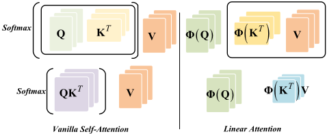
Linear Attention. Vanilla self-attention employs the Softmax function on a row-wise basis within the attention matrix, leading to competition among values in the same row, as depicted in Figure 3(a). In contrast, linear attention does not face such constraints. As shown in Figure 4, linear attention can be expressed as Φ (Q) Φ (K) 𝑇 V, where Φ (·) is the mapping function. As shown in Figure 3, linear attention demonstrates better attention matrix shaping capabilities. Quantitative results can be found in Table 5.
The mapping function directly impacts the focusing capability and overall performance of linear attention. Herein we introduce a novel learnable mapping function:
where Softmax is applied row-wise to the input matrix, and 𝜏 is a learnable parameter to adjust dynamically the Softmax temperature. Note that in Eq. 4, the Softmax function is applied to the matrices Q and K, rather than directly to the attention matrix, as is the case with vanilla selfattention. This distinction is fundamental to the increased flexibility of the attention matrix. Moreover, we set all negative values in the matrices Q and K to a large negative number, such as -100, to ensure that these values are close to 0 after applying the mapping function. Various mapping functions have been explored in prior research, including the power function [Han et al., 2023], column-wise Softmax [Shen et al., 2021], ReLU [Cai et al., 2023], and elu function [Katharopoulos et al., 2020]. Our empirical experiments demonstrate the effectiveness of our mapping function in time series anomaly detection, as detailed in Table 5.
3.3 Loss Function and Anomaly Score
Loss Function. Reconstruction loss is fundamental in unsupervised time series anomaly detection. As aforementioned, we also introduce the sub-adjacent attention contribution into the loss function, which guides the model to focus on the sub-adjacent neighborhoods. By integrating these two losses, the loss function for the input series X ∈ R 𝑇×𝐷 is formulated as follows:
where Lrec is the reconstruction loss and Lattn is the attention loss, λ > 0 is the weight to trade off the two terms. ∥·∥𝐹 and ∥·∥1 in Eq. 5 are the Frobenius and k-norm, respectively. ˆX ∈ R 𝑇×𝐷 denotes the reconstructed X.
Anomaly Score. To identify anomalies, we combine the sub-adjacent attention contribution with the reconstruction errors. Consistent with with the approach in [Xu et al., 2022], the Softmax function is applied to -SACon (A) to highlight the anomalies with less attention contribution. Subsequently, we perform an element-wise multiplication of the attention results and reconstruction errors. Finally, the anomaly score for each point can be expressed as
where ⊙ is the element-wise multiplication. Typically, the anomalies exhibit less attention contribution and higher reconstruction errors, leading to larger anomaly scores.
Dynamic Gaussian Scoring. Following the practice of [Schmidl et al., 2022], we fit a dynamic Gaussian distribution to anomaly scores obtained by Eq. 6 and design a score based on the fitted distribution. Let 𝜇𝑡 and 𝜎𝑡 denote the dynamic mean and standard variance, respectively, which can be computed in the way of sliding windows. Then the final score with dynamic Gaussian fitting can be computed via
| Dataset | Dims | Entities | #Train (K) | #Test (K) | AR (%) |
|---|---|---|---|---|---|
| SWaT | 51 | 1 | 495 | 449 | 12.14 |
| WADI | 123 | 1 | 1209 | 172 | 5.71 |
| PSM | 25 | 1 | 132 | 87 | 27.76 |
| MSL | 55 | 27 | 58 | 73 | 10.48 |
| SMAP | 25 | 55 | 140 | 444 | 12.83 |
| SMD | 38 | 28 | 708 | 708 | 4.16 |
| NeurIPS-TS | 1 | 1 | 20 | 20 | 22.44 |
where cdf is the cumulative distribution function of the standard Gaussian distribution 𝑁 (0, 1).
4 Experiments
4.1 Datasets
We evaluate the Sub-Adjacent Transformer on the following datasets, whose statistics are summarized in Table 1.
SWaT (Secure Water Treatment) [Mathur and Tippenhauer, 2016] is collected continuously over 11 days from 51 sensors located at a water treatment plant. WADI (WAter DIstribution) [Ahmed et al., 2017] is acquired from 123 sensors of a reduced water distribution system for 16 days. PSM (Pooled Server Metrics) [Abdulaal et al., 2021] is collected from multiple servers at eBay with 26 dimensions. MSL (Mars Science Laboratory rover) and SMAP (Soil Moisture Active Passive satellite) are datasets released by NASA with 55 and 25 dimensions respectively. SMD (Server Machine Dataset) [Su et al., 2019] is collected from a large compute cluster, consisting of 5 weeks of data from 28 server machines with 38 sensors. NeurIPS-TS (NeurIPS 2021 Time Series Benchmark) is a synthetic dataset proposed by [Lai et al., 2021] and includes 5 kinds of anomalies that cover pointand pattern-wise behaviors: global (point), contextual (point), shapelet (pattern), seasonal (pattern), and trend (pattern).
4.2 Implementation Details
Following the common practice, we adopt a non-overlapping sliding window mechanism to obtain a series of sub-series. The sliding window size is set as 100 without particular statements. 𝐾1 and 𝐾2 are set as 20 and 30, respectively. The choices of these parameters will be discussed later in ablation studies. The points are judged to be anomalies if their anomaly scores (Eq. 7) are larger than a certain threshold 𝛿. In this study, following the practice of paper [Lai et al., 2023; Xu et al., 2022], the thresholds are chosen to output the best F1 scores. The widely-used point adjustment strategy [Xu et al., 2022; Tuli et al., 2022; Garg et al., 2022;
| Category | Single-Entity | Multi-Entity† | ||||||||||
|---|---|---|---|---|---|---|---|---|---|---|---|---|
| Datset | SWaT | WADI | PSM | MSL | SMAP | SMD | ||||||
| Metric | AUC | F1 | AUC | F1 | AUC | F1 | AUC | F1 | AUC | F1 | AUC | F1 |
| DAGMM [2018] | 91.6 | 85.3 | 29.2 | 20.9 | 85.2 | 76.1 | 80.6 | 70.1 | 81.5 | 71.2 | 82.3 | 72.3 |
| LSTM-VAE [2018] | 88.3 | 80.5 | 49.8 | 38.0 | 88.6 | 80.9 | 91.6 | 85.4 | 84.8 | 75.6 | 88.6 | 80.8 |
| MSCRED [2019] | 88.5 | 80.7 | 49.1 | 37.4 | 74.3 | 62.6 | 96.6 | 93.6 | 92.4 | 86.6 | 90.8 | 84.1 |
| OmniAnomaly [2019] | 92.4 | 86.6 | 53.9 | 41.7 | 77.6 | 66.4 | 94.6 | 90.1 | 91.6 | 85.4 | 98.0 | 96.2 |
| MAD-GAN [2019] | 89.0 | 81.5 | 67.9 | 55.6 | 77.1 | 65.8 | 95.5 | 91.7 | 92.3 | 86.5 | 95.4 | 91.5 |
| MTAD-GAT [2020] | 92.0 | 86.0 | 72.2 | 60.2 | 86.6 | 78.0 | 95.0 | 90.8 | 94.6 | 90.1 | 95.0 | 90.8 |
| USAD [2020] | 91.1 | 84.6 | 55.3 | 43.0 | 82.5 | 72.5 | 95.2 | 91.1 | 89.3 | 81.9 | 97.2 | 94.6 |
| THOC [2020] | 93.3 | 88.1 | 63.1 | 50.6 | 94.2 | 89.5 | 96.7 | 93.7 | 97.5 | 95.2 | 66.5 | 54.1 |
| UAE [2022] | 92.6 | 86.9 | 97.8 | 95.7 | 96.6 | 93.6 | 95.7 | 92.0 | 94.3 | 89.6 | 98.6 | 97.2 |
| GDN [2021] | 96.5 | 93.5 | 91.7 | 85.5 | 95.9 | 92.3 | 94.7 | 90.3 | 81.1 | 70.8 | 81.8 | 71.6 |
| GTA [2021] | 95.1 | 91.0 | 90.7 | 84.0 | 91.7 | 85.5 | 95.2 | 91.1 | 94.7 | 90.4 | 95.6 | 91.9 |
| TranAD [2022] | 89.0 | 81.5 | 62.0 | 49.5 | 93.4 | 88.2 | 97.3 | 94.9 | 94.0 | 89.2 | 98.0 | 96.1 |
| Heuristics [2022] | 98.4 | 96.9 | 98.2 | 96.5 | 99.2 | 98.5 | 98.2 | 96.5 | 98.0 | 96.1 | 96.5 | 93.4 |
| Anomaly Transformer [2022] | 96.9 | 94.1 | 98.3 | 96.6 | 98.9 | 97.9 | 96.6 | 93.6 | 98.3 | 96.7 | 95.9 | 92.3 |
| NPSR [2023] | 97.5 | 95.3 | 96.7 | 93.8 | 97.8 | 95.7 | 97.9 | 96.0 | 98.9 | 97.8 | 91.4 | 85.0 |
| TimesNet [2023] | - | 92.1 | - | - | - | 97.5 | - | 85.2 | - | 71.5 | - | 85.8 |
| Ours | 99.5 | 99.0 | 99.7 | 99.3 | 99.4 | 98.9 | 98.3 | 96.7 | 99.1 | 98.2 | 98.7 | 97.7 |
| Methods | DAGMM [2018] | LSTM-VAE [2018] | OmniAnomaly [2019] | THOC [2020] | Heuristics [2022] | Anomaly Transformer [2022] | NPSR [2023] | TimesNet [2023] | Ours |
|---|---|---|---|---|---|---|---|---|---|
| AUC | 64.3 | 70.5 | 72.2 | 74.2 | 85.5 | 86.2 | 76.7 | 79.6 | 92.4 |
| F1 | 51.8 | 58.4 | 60.2 | 62.5 | 76.3 | 77.5 | 65.4 | 69.5 | 86.6 |
Wu et al., 2023] is adopted. Note that point adjustment has its practicality: one detected anomaly point will guide system administrators to identify the entire anomalous segment. The Sub-Adjacent Transformer contains 3 layers. Specifically, we set the hidden dimension 𝑑model as 512, and the head number as 8. The hyper-parameter λ as 10 in Eq. 5 to balance recognition loss and attention loss. The Adam optimizer [Kingma and Ba, 2015] is used with an initial learning rate of 10 -4 . Following [Xu et al., 2022], the training is early stopped within 10 epochs with the batch size of 128. Experiments are conducted using PyTorch and one NVIDIA RTX A6000 GPU.
4.3 Main Results
Real-World Datasets. In Table 2, we report AUC and F1 metrics for various methods on six real-world datasets with 15 competitive baselines. The Sub-Adjacent Transformer consistently achieves state-of-the-art performance across all benchmarks, with an average improvement of 1.7 and 0.4 percentage points in F1 score over the current SOTA for singleentity and multi-entity datasets, respectively. Note that for multi-entity datasets, we combine all entities and train them together using a single model, whereas some methods, such as simple heuristics [Garg et al., 2022] and NPSR [Lai et al., 2023], train each entity separately and average the results. Even though entity-to-entity variations are large (especially MSL and SMD datasets), the Sub-Adjacent Transformer still achieves better anomaly detection results using one model than the multi-model counterpart, showing the advantage of the proposed attention mechanism. We have retained all dimensions of the original datasets, even though some of them are constant and do not play a role. Additionally, we also report F1 results without using point-adjustment in the supplementary material, where the Sub-Adjacent Transformer also exhibits competitive performance.
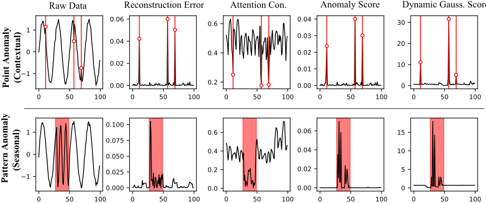
Synthetic Dataset. NeurIPS-TS is a challenging synthetic dataset. We generate the NeurIPS-TS dataset using the source codes released by [Lai et al., 2021], and it includes 5 anomalous types covering both the point-wise (global and contextual) and pattern-wise (shapelet, seasonal and trend) anomalies. As shown in Table 3, the Sub-Adjacent Transformer achieves state-of-the-art performance with an astonishing 9.1 percentage points improvement of F1 score relative to Anomaly Transformer [Xu et al., 2022], demonstrating the effectiveness of the proposed model on various anomalies. Visualization results can be found in Figure 5. We can see that anomalies do have less sub-adjacent contribution (the third column), which is consistent with our assumption. A full version of Figure 5 can be found in the supplementary material.
| 𝐾1 : 𝐾2 | SWaT | WADI | PSM | MSL | SMAP | SMD |
| 0 : 0 | 94.8 | 93.5 | 95.3 | 91.5 | 92.4 | 93.8 |
| 0 : 5 | 96.7 | 95.9 | 97.6 | 93.6 | 93.7 | 94.1 |
| 0 : 10 | 98.5 | 98.2 | 98.7 | 94.4 | 96.9 | 95.9 |
| 10 : 20 | 97.6 | 98.1 | 98.1 | 96.5 | 97.8 | 94.4 |
| 20 : 30 | 99.0 | 99.3 | 98.9 | 96.7 | 98.2 | 97.7 |
| 30 : 40 | 97.6 | 94.8 | 97.8 | 95.6 | 97.5 | 94.0 |
| 10 : 30 | 97.8 | 97.8 | 98.8 | 95.0 | 97.4 | 94.5 |
| 20 : 40 | 97.9 | 98.0 | 93.5 | 95.7 | 95.6 | 94.4 |
| 10 : 40 | 98.0 | 97.7 | 98.7 | 96.1 | 97.5 | 97.8 |
4.4 Ablation Studies
Vanilla and Linear Transformer. We compare vanilla self-attention and linear attention with different mapping functions using our method. As shown in Table 5, the proposed Softmax-based mapping function with learnable parameters outperforms other mapping functions and vanilla self-attention, with a maximum F1 score increase of 1.5 percentage points.
Choices of 𝐾1 and 𝐾2. Choices of 𝐾1 and 𝐾2 directly affect the performance of the Sub-Adjacent Transformer. We evaluate the effect in Table 4 with the window size being 100. The configuration of 𝐾1 = 20 and 𝐾2 = 30 typically yields the best performance (with the exception of the SMD dataset), while the performance of other settings is also satisfactory, with nearly half of the values exceeding the current SOTA. When the sub-adjacent span is getting close to the diagonal (the second and third rows in Table 4), the performance worsens. We also explore the extreme case where 𝐾1 = 𝐾2 = 0. In that case, the performance drops significantly, highlighting the importance of sub-adjacent attention.
Module Ablation. We evaluate the contribution of linear attention module and dynamic scoring module in Table 6. For the Sub-Adjacent Transformer, the baseline means the proposed sub-adjacent attention mechanism accompanied with vanilla self-attention and anomaly score (Eq. 6). Then linear attention and Gaussian dynamic scoring (Eq. 7) are introduced in turn. As shown in Table 6, compared with the baseline, linear attention brings +1.0 improvement on average over six datasets and Gaussian dynamic scoring brings another +0.2 improvement, verifying the effectiveness of the proposed modules.
Furthermore, we also apply the two modules to Anomaly Transformer [Xu et al., 2022]. As we can see from Table 6, the proposed linear attention model provides +1.2 percentage points performance gain averagely, and Gaussian dynamic scoring provides another +0.1 gain. Moreover, as shown in Table 6, without the support of linear attention and dynamic Gaussian score, our method (baseline) still outperforms the Anomaly Transformer by an average of +1.8 percentage points, thereby validating the efficacy of our subadjacent attention design.
| Dataset | SWaT | WADI | PSM | MSL | SMAP | SMD | |
|---|---|---|---|---|---|---|---|
| Vanilla self-attention [Vaswani et al., 2017] | 98.6 | 98.2 | 98.8 | 94.1 | 97.4 | 96.5 | |
| Softmax column [Shen et al., 2021] | 98.0 | 97.5 | 96.9 | 95.2 | 97.8 | 95.8 | |
| Attn. | Power function [Han et al., 2023] | 98.4 | 98.3 | 98.4 | 93.7 | 97.5 | 95.9 |
| Lin. ReLU [Cai | et al., 2023] | 98.8 | 98.1 | 97.6 | 94.3 | 97.5 | 94.8 |
| ELU+1 [Katharopoulos et al., 2020] | 95.4 | 95.6 | 94.1 | 94.7 | 96.3 | 94.5 | |
| Ours (Eq. 4) | 99.0 | 99.3 | 98.9 | 96.7 | 98.2 | 97.7 | |
| Baseline | Linear Attention | Dynamic Scoring | SWaT | WADI | PSM | MSL | SMAP | SMD | |
|---|---|---|---|---|---|---|---|---|---|
| Ours | ✓ | 98.2 | 98.0 | 98.7 | 93.9 | 97.0 | 96.1 | ||
| ✓ | ✓ | 98.8(+0.6) | 99.1(+1.1) | 98.8(+0.1) | 96.4(+2.5) | 97.9(+0.9) | 97.0(+0.9) | ||
| ✓ | ✓ | ✓ | 99.0(+0.8) | 99.3(+1.3) | 98.9(+0.2) | 96.7(+2.8) | 98.2(+1.2) | 97.7(+1.6) | |
| Anomaly | ✓ | 94.1 | 96.6 | 97.9 | 93.6 | 96.7 | 92.3 | ||
| Transformer | ✓ | ✓ | 98.1(+4.0) | 97.6(+1.0) | 98.3(+0.4) | 93.6(+0.0) | 97.6(+0.9) | 93.4(+1.1) | |
| [2022] | ✓ | ✓ | ✓ | 98.3(+4.2) | 97.9(+1.3) | 98.2(+0.3) | 93.7(+0.1) | 97.7(+1.0) | 93.6(+1.3) |
| W S | SWaT | WADI | PSM | MSL | SMAP | SMD |
|---|---|---|---|---|---|---|
| 50 | 97.6 | 97.8 | 98.4 | 94.7 | 96.9 | 92.1 |
| 100 | 99.0 | 99.3 | 98.9 | 96.7 | 98.2 | 97.7 |
| 150 | 98.8 | 98.8 | 98.7 | 94.9 | 97.3 | 96.4 |
| 200 | 99.1 | 98.7 | 98.5 | 94.9 | 97.5 | 94.2 |
| 250 | 97.2 | 98.1 | 98.3 | 95.3 | 97.4 | 93.9 |
| 300 | 98.9 | 98.2 | 98.1 | 94.3 | 96.9 | 94.3 |
Choices ofWindow Size. Table 7 gives F1 values with different window sizes for six datasets. One can see that our model exhibits good robustness to the window size. The optimal performance is typically achieved with a window size of 100, the only exception being the SWaT dataset.
Choices of Parameter λ. Table 8 compares the performance for different values of λ. The best results are achieved when λ is set to 10, while the second-best results occur at different values of λ for different datasets. It is noteworthy that without the inclusion of attention loss (λ = 0), performance drops drastically, affirming the effectiveness of our sub-adjacent attention design.
| λ | SWaT | WADI | PSM | MSL | SMAP | SMD |
|---|---|---|---|---|---|---|
| 0 | 95.8 | 94.2 | 95.6 | 92.7 | 95.3 | 94.8 |
| 4 | 98.8 | 97.8 | 98.8 | 94.7 | 97.6 | 96.7 |
| 6 | 98.6 | 98.3 | 98.6 | 96.1 | 97.4 | 97.3 |
| 8 | 98.3 | 97.8 | 98.7 | 95.8 | 98.0 | 96.9 |
| 10 | 99.0 | 99.3 | 98.9 | 96.7 | 98.2 | 97.7 |
| 12 | 98.5 | 98.3 | 98.6 | 95.8 | 97.6 | 97.1 |
| 14 | 98.7 | 98.2 | 98.6 | 95.2 | 97.3 | 96.3 |
5 Conclusion
In this paper, we present the Sub-Adjacent Transformer, a novel paradigm for utilizing attention in time series anomaly detection. Our method distinctively combines sub-adjacent attention contribution, linear attention and reconstruction error to effectively detect anomalies, thereby enhancing the efficacy of anomaly detection. It offers a novel perspective on the utilization of attention in this domain. Without bells and whistles, our model demonstrates superior performance across common benchmarks. We hope that the Sub-Adjacent Transformer could act as a baseline framework for the future works in time series anomaly detection.
Acknowledgments
This work was supported by the National Science Foundation of China (NSFC) (No. 62371009 and No. 61971008).
@inproceedings{ijcai2024p279,
  title     = {Sub-Adjacent Transformer: Improving Time Series Anomaly Detection with Reconstruction Error from Sub-Adjacent Neighborhoods},
  author    = {Yue, Wenzhen and Ying, Xianghua and Guo, Ruohao and Chen, DongDong and Shi, Ji and Xing, Bowei and Zhu, Yuqing and Chen, Taiyan},
  booktitle = {Proceedings of the Thirty-Third International Joint Conference on
               Artificial Intelligence, {IJCAI-24}},
  publisher = {International Joint Conferences on Artificial Intelligence Organization},
  editor    = {Kate Larson},
  pages     = {2524--2532},
  year      = {2024},
  month     = {8},
  note      = {Main Track},
  doi       = {10.24963/ijcai.2024/279},
  url       = {https://doi.org/10.24963/ijcai.2024/279},
}
TY - CPAPER TI - Sub-Adjacent Transformer: Improving Time Series Anomaly Detection with Reconstruction Error from Sub-Adjacent Neighborhoods AU - Yue, Wenzhen AU - Ying, Xianghua AU - Guo, Ruohao AU - Chen, DongDong AU - Shi, Ji AU - Xing, Bowei AU - Zhu, Yuqing AU - Chen, Taiyan T2 - Proceedings of the Thirty-Third International Joint Conference on Artificial Intelligence, IJCAI-24 PB - International Joint Conferences on Artificial Intelligence Organization PY - 2024 SP - 2524 EP - 2532 DO - 10.24963/ijcai.2024/279 UR - https://doi.org/10.24963/ijcai.2024/279 ER -Copied
Machine-readable versions of this paper, for tools and AI agents:





