
Sampling Winners in Ranked Choice Voting
Proceedings of the Thirty-Third International Joint Conference on Artificial Intelligence. Main Track. Pages 2834-2841.
https://doi.org/10.24963/ijcai.2024/314
Keywords
- Game Theory and Economic Paradigms: GTEP: Computational social choice
Abstract
Ranked choice voting (RCV) is a voting rule that iteratively eliminates least-popular candidates until there is a single winner with a majority of all remaining votes. In this work, we explore three central questions about predicting the outcome of RCV on an election given a uniform sample of votes. First, in theory, how poorly can RCV sampling predict RCV outcomes? Second, can we use insights from the recently-proposed map of elections to better predict RCV outcomes? Third, is RCV the best rule to use on a sample to predict the outcome of RCV in real-world elections? We find that although RCV can do quite poorly in the worst case and it may be better to use other rules to predict RCV winners on synthetic data from the map of elections, RCV generally predicts itself well on real-world data, further contributing to its appeal as a theoretically-flawed but practicable voting process. We further supplement our work by exploring the effect of margin of victory (MoV) on sampling accuracy.
- [Arora et al., 2012] Sanjeev Arora, Elad Hazan, and Satyen Kale. The multiplicative weights update method: a meta-algorithm and applications. Theory of computing, 8(1):121-164, 2012.
- [Bhattacharyya and Dey, 2021] Arnab Bhattacharyya and Palash Dey. Predicting winner and estimating margin of victory in elections using sampling. Artificial Intelligence, 296:103476, 2021.
- [Boehmer and Schaar, 2023] Niclas Boehmer and Nathan Schaar. Collecting, classifying, analyzing, and using real- world elections. In Proceedings of the 22nd International Conference on Autonomous Agents and Multi-Agent Sys- tems (AAMAS), pages 1706-1715, 2023.
- [Boehmer et al., 2021] Niclas Boehmer, Robert Bredereck, Piotr Faliszewski, Rolf Niedermeier, and Stanisław Szufa. Putting a compass on the map of elections. In Proceedings of the 30th International Joint Conference on Artificial In- telligence (IJCAI), pages 59-65, 2021. IJCAI
- [Boehmer et al., 2023] Niclas Boehmer, Jin-Yi Cai, Piotr Faliszewski, Austen Z Fan, Łukasz Janeczko, Andrzej Kaczmarczyk, and Tomasz Was. Properties of position matrices and their elections. In The 37th AAAI Conference on Artificial Intelligence (AAAI), pages 5507-5514, 2023.
- [Brandt et al., 2016] Felix Brandt, Vincent Conitzer, Ulle Endriss, Jérôme Lang, and Ariel D Procaccia. Handbook of computational social choice. Cambridge University Press, 2016.
- [Cary, 2011] David Cary. Estimating the margin of vic- tory for instant-runoff voting. In 2011 Electronic Voting Technology Workshop/Workshop on Trustworthy Elections (EVT/WOTE 11), 2011.
- [Dey and Narahari, 2015] Palash Dey and Yadati Narahari. Estimating the margin of victory of an election using sam- pling. In Proceedings of the 24th International Joint Conference on Artificial Intelligence (IJCAI), pages 1120- 1126, 2015. IJCAI
- [Donovan et al., 2019] Todd Donovan, Caroline Tolbert, and Kellen Gracey. Self-reported understanding of ranked- choice voting. Social Science Quarterly, 100(5):1768- 1776, 2019.
- [Faliszewski et al., 2019] Piotr Faliszewski, Piotr Skowron, Arkadii Slinko, Stanisław Szufa, and Nimrod Talmon. How similar are two elections? In Proceedings of the AAAI Conference on Artificial Intelligence, volume 33, pages 1909-1916, 2019.
- [Felsenthal and Tideman, 2013] Dan S Felsenthal and Nico- laus Tideman. Varieties of failure of monotonicity and par- ticipation under five voting methods. Theory and Decision, 75:59-77, 2013.
- [Graham-Squire and McCune, 2023] Adam Graham-Squire and David McCune. An examination of ranked-choice vot- ing in the united states, 2004-2022. Representation, pages 1-19, 2023. [Harvard, 2020] Harvard. Harvard Dataverse. https: //dataverse.harvard.edu/dataset.xhtml?persistentId=doi: 10.7910/DVN/AMK8PJ, 2020. Accessed: 2023-09-06. DOI
- [Horton and Thomas, 2023] Jennifer Horton and Dakota Thomas. Ranked choice voting: What, where, why & why not, 2023.
- [Kizilkaya and Kempe, 2022] Fatih Erdem Kizilkaya and David Kempe. Plurality veto: A simple voting rule achieving optimal metric distortion. arXiv preprint arXiv:2206.07098, 2022. IJCAI
- [Littlestone and Warmuth, 1994] Nick Littlestone and Man- fred K Warmuth. The weighted majority algorithm. Infor- mation and computation, 108(2):212-261, 1994.
- [Mattei and Walsh, 2013] Nicholas Mattei and Toby Walsh. Preflib: A library for preferences http://www. preflib. org. In Algorithmic Decision Theory: Third International Con- ference, ADT 2013, Bruxelles, Belgium, November 12-14, 2013, Proceedings 3, pages 259-270. Springer, 2013. Link
- [Micha and Shah, 2020] Evi Micha and Nisarg Shah. Can we predict the election outcome from sampled votes? In Proceedings of the 34th AAAI Conference on Artificial In- telligence (AAAI), pages 2176-2183, 2020.
- [Spencer et al., 2015] Andrew Spencer, Christopher Hughes, and Rob Richie. Escaping the thicket: The ranked choice voting solution to america's redistricting crisis. Cumb. L. Rev., 46:377, 2015.
- [Szufa et al., 2020] Stanislaw Szufa, Piotr Faliszewski, Piotr Skowron, Arkadii M. Slinko, and Nimrod Talmon. Draw- ing a map of elections in the space of statistical cultures. In Proceedings of the 19th International Conference on Autonomous Agents and Multi-Agent Systems (AAMAS), pages 1341-1349, 2020.
- [Tolbert and Kuznetsova, 2021] Caroline Tolbert and Daria Kuznetsova. Editor's introduction: The promise and peril of ranked choice voting. Politics and Governance, 9(2):265-270, 2021.
References were extracted automatically from the PDF and may contain errors.
Full text extracted automatically from the PDF; figures, tables and equations may differ. The PDF is the version of record.
1 Introduction
Democratic systems elicit and aggregate opinions from citizens in order to make collective decisions. The most common way in which they do this is through voting, in which citizens provide structured feedback via ballots, which are then aggregated via a social choice function, also called a voting rule, in order to determine a winner.
One such rule is ranked choice voting (RCV), also known as instant-runoff voting (IRV), single transferable vote (STV), or preferential voting [Spencer et al., 2015]. RCV, or variants thereof, is used in political elections around the world, including Australia, Ireland, New Zealand, and the United States, for a mixture of federal, parliamentary, and local elections. In the United States in particular, RCV is championed by activist groups like FairVote to replace the use of first-pastthe-post voting systems and is currently used by 11 million residents: Alaska and Maine use RCV for federal and/or local elections, and an additional 53 cities use RCV for local elections, including New York City's Democractic primary for the mayoral election in 2021 [Horton and Thomas, 2023].
Despite significant activist support for RCV and increasing adoption worldwide, RCV is known to have significant theoretical flaws, notably for being susceptible to monotonicity paradoxes [Felsenthal and Tideman, 2013]. However, in practice, real-world elections do not often resemble worst-case constructions or even synthetic elections generated from statistical cultures [Boehmer and Schaar, 2023], and RCV generally performs well [Graham-Squire and McCune, 2023].
One major concern expressed by activists pushing for more widespread adoption of RCV is that of predicting the outcomes of RCV elections from sampled votes, especially because RCV outcomes can change so drastically as new votes are counted. Our goal is to study how to predict outcomes in RCV elections from samples.
In this work, we aim to explore three central questions about predicting RCV outcomes in sampled elections. First, in the worst case over voting profiles, how poorly can RCV on a sample predict the outcome of RCV on the entire election? Second, can we use insights from elections generated from well-studied statistical cultures to better predict RCV outcomes? And third, how well does RCV predict itself on samples from real-world elections?
1.1 Our Contributions
We begin by examining the worst-case predictive performance of RCV in theory. Surprisingly, we show that, in theory, this performance seems to decrease as the sample size grows: For samples of size 1, we obtain a tight bound of probability at least 1/2m-1 of making the correct decision, 1 but for samples consisting of all but a constant number of votes in the election, we are able to create worst-case instances such that the predictive performance of RCV drops to 0, i.e., using RCV on the sample never yields the same result as evaluating RCV on the entire profile. Additionally, we provide upper bounds on the minimum sample size necessary to guarantee a correct prediction in terms of the margin of victory of the original election, where the margin of victory is defined as the total number of votes that must be changed in order to change the winner of the election.
Next, we examine the performance of a collection of nine voting rules predicting RCV outcomes on synthetic elections generated from a diverse set of statistical cultures from the map of elections [Szufa et al., 2020; Boehmer et al., 2021]. We observe that, especially on small sample sizes, RCV is often not the best predictor of itself and that other rules are more reliable.
1 Following convention, m is the number of alternatives.
However, this observation does not hold as strongly for real-world elections. On a range of elections sourced from PrefLib, we find that, on average, RCV is generally the best predictor of itself even on small sample sizes. This does not hold for every individual election, but RCV is even comparable to two ensemble predictors that use the map of elections to boost performance.
1.2 RelatedWork
The paper most closely related to ours is that of Micha and Shah [2020], which studies the worst- and average-case predictability of social welfare functions (SWFs), which return rankings over candidates instead of winner(s). The authors focus on positional scoring rules (PSRs) and demonstrate that all PSRs except plurality and veto have zero worst-case predictability even with access to a sample of as many as n - 1 out of n votes. They also include an empirical section that evaluates how well various SWFs can predict each other on two synthetic vote distributions. In our work, we focus on predicting social choice functions (SCFs), in particular RCV; we also consider a significantly more diverse collection of both synthetic and real-world data.
The synthetic data we use is directly inspired (and generated) by the map of elections [Faliszewski et al., 2019; Szufa et al., 2020; Boehmer et al., 2021], which is a principled approach to generating, organizing, and visualizing a diverse set of statistical cultures from which to generate realistic election data.
Another related theoretical paper is that of Bhattacharyya and Dey [2021], where the authors focus on predicting the output of a SCF on an unknown profile through sampling votes. However, the authors assume that votes are sampled with replacement and that there is a margin of victory of at least αn for some constant α. We do not make such assumptions in our worst-case results, and indeed our negative results come in borderline cases. We do consider the margin of victory in RCV elections in our work on bounding the number of samples necessary to make perfect predictions, which draws on work by Cary [2011] and Dey and Narahari [2015].
Further afield, there is also significant theoretical and empirical work on paradoxes in STV [Graham-Squire and McCune, 2023; Tolbert and Kuznetsova, 2021; Donovan et al., 2019], but this work does not focus on sampling.
2 Preliminaries
Let [n] := {1, . . . , n}. Let A = {a1, . . . , am} be a set of m alternatives and N = [n] be a set of n voters. Let L(A) be the set of all complete and incomplete rankings over A, i.e., (partial) permutations of all alternatives. Each voter i ∈ N casts a vote σi ∈ L(A). The collection of all n votes is the profile ⃗σ = (σ1, . . . , σn). We use the notation aj ≻i ak to denote that voter i prefers aj to ak and drop the voter subscript when the voter identity is clear.
We focus on social choice functions (SCFs) (here interchangeably referred to as voting rules), which are functions f : L(A)n → A that, given an input profile, output a winner of the election. 2 Let sg(n) denote a sample taken uniformly at random and without replacement from a complete profile ⃗σ such that |sg(n)| = g(n) for a function g : N → N which, given a number of voters n, returns a sample size in [n]. We use sg(n) ∼ ⃗σ to denote this process of uniformly selecting a sample sg(n) without replacement from ⃗σ. When g(n) is clear, we let s := sg(n) for brevity.
We also define the worst-case accuracy of a rule f predicting a rule f ′ given a sampling function g and a maximum number of alternatives m as
Intuitively, this is the minimum probability of f correctly predicting f ′ on a sample for profiles that consist of exactly m0 alternatives as n becomes large. When f = f ′ , we let Af(g,m0) := Af,f ′(g,m0) for brevity.
2.1 Voting Rules
We define the voting rules in this paper, namely RCV, plurality, Borda, harmonic, Copeland, Minimax, Bucklin, Plurality Veto, and veto, which are discussed in greater detail in [Brandt et al., 2016; Kizilkaya and Kempe, 2022].
RCV proceeds in rounds as follows. In each of m - 1 rounds, each candidate counts the total number of first-place votes they have, and the candidate with the fewest first-place votes is eliminated. 3 All voters who selected the eliminated candidate as their most-preferred candidate move on to their next most preferred candidate. If, in the course of candidate eliminations, a particular vote has no active candidates remaining, the vote is removed from the election. 4 This process terminates with a single winner. Additionally, it is easy to see that if any candidate has a majority of all first-place votes at any stage of the process, that candidate will win the election.
Plurality, Borda, harmonic, and Veto are all instances of positional scoring rules (PSRs). PSRs are characterized by a scoring vector ⃗c = (c1, . . . , cm) ∈ Rm, where cj ≥ cj+1 for all j ∈ {1, . . . , m-1} and c1 > cm. Given a profile ⃗σ, a PSR with scoring vector ⃗c assigns a score sc(aj) = ∑ni=1 cσi(aj), where σi(aj) is the position of aj in voter i's ranking, σi. The alternative with the highest score is the winner.
The scoring vectors of the four rules are as follows: Plurality uses ⃗c = (1, 0, . . . , 0), Borda uses ⃗c = (m - 1,m - 2, . . . , 0), harmonic uses ⃗c = (1, 1/2, . . . , 1/m), and veto uses ⃗c = (0, . . . , 0, -1).
The Copeland rule and Minimax both consider pairwise comparisons between alternatives. The Copeland rule chooses the alternative that beats the greatest number of other alternatives in head-to-head comparisons 5 , and Minimax chooses the alternative that has the smallest maximum margin of defeat in all head-to-head comparisons.
2 Although SCFs may return sets of winners, we use tiebreaking procedures to choose a single winner. In our theoretical results, we use lexicographic tiebreaking. In our empirical results, we break ties uniformly at random due to our method of vote completion.
3 Tiebreaking occurs in each round of RCV.
4 This occurs when voters submit incomplete preferences.
5 Head-to-head ties count as half a win.
Bucklin starts with all first-place votes and iteratively adds second-place votes, third-place votes, and so on until an alternative reaches a majority of all votes counted so far; that alternative is returned as the winner. Plurality Veto [Kizilkaya and Kempe, 2022] decrements each alternative's plurality score through n rounds of a veto process, taken in a randomly permuted order, and the last remaining candidate wins.
3 Worst-Case Accuracy of RCV
Somewhat paradoxically, we find that the worst-case accuracy of RCV seems to decrease as we increase the size of the sample we take. However, as we will see in the empirical section, this trend is reversed in practice.
Throughout this section, we will analyze RCV with lexicographic (i.e., alphabetical) tiebreaking where, for instance, a1 defeats a2 if they are tied. All missing proofs are included in the full version. 6
3.1 Sampling a Single Vote
We begin our analysis in the case of |s| = 1, i.e., with samples consisting of only a single vote from the profile. In this case, we can show a tight bound on the probability that RCV predicts itself correctly.
Proof. We first show the upper bound: AR(g,m) ≤ 1 2m-1 . Consider the following profile:
Here, the notation c : σi means that c voters have the preference σi. In this scenario, a1 wins the election and starts with only 1 vote, which is 1 2m-1 of the votes in the election. Therefore, RCV predicts itself correctly with probability 1 2m-1 . This profile can be multiplied to create arbitrarily large elections in which this holds.
Now, we show the matching lower bound: AR(g,m) ≥ 1 2m-1 . Note that this proof works for profiles in which all ballots have complete rankings, but it is possible to modify it to work with incomplete rankings as well; see the full version of the paper. Running RCV on a single ballot selects that ballot's first choice as the winner, so the question of finding the worst case probability of RCV predicting itself correctly on a single randomly selected ballot is exactly the same as determining how small we can make the portion of ballots that select the true RCV winner, a∗ , as the first choice. Let vk(ai) represent the number of first choice votes that alternative ai receives in round k. For all k ∈ [2,m- 1], we know that vk(ai) ≤ 2vk-1(ai) for all ai not eliminated by round k because the losing candidate of round k - 1 always has the fewest first choice votes in that round, so any other candidate cannot more than double their first place vote share from one round to the next. We also know that by the final round, i.e., round m- 1, the RCV winner a∗ must have at least half of all votes. Therefore, vm-1(a∗ ) ≥ n/2. Now, applying the relation above, we see that v1(a∗ ) ≥ 12 v2(a∗ ) ≥ · · · ≥ 1 2m-3 vm-2(a∗ ) ≥ 1 2m-2 vm-1(a∗ ) ≥ n 2m-1 , as desired.
6 The full version is available at https://ansonkahng.com/.
3.2 Sampling All but k Votes
We now move to the other end of the sample size spectrum and ask how well RCV can predict itself given access to almost all of the votes in a profile. Intuitively, it seems like having access to more votes should only help the accuracy of RCV when predicting itself, but we will see that this is not necessarily the case.
Our next theorem states that, even with all but one sample from a profile, RCV's worst-case predictive accuracy is 0, i.e., there exist profiles such that running RCV on any sample of all but one vote returns a different winner than running RCV on the entire profile.
Proof. For as few as four candidates, it is possible to construct arbitrarily large profiles in which sampling every ballot but one always yields the incorrect result. Consider the following election:
One can verify that a1 wins in this profile. Despite this, when we sample all but one vote, if the missing vote has a first choice other than a4, a4 ends up winning, and otherwise when we remove a ballot with a4 as a first choice, a2 ends up winning. When we scale up this profile to larger sizes by multiplying the number of each ballot by some constant, this property remains, so we can construct arbitrarily large elections in which sampling all but one vote and performing RCV never yields the true winner of the election.
Lastly, in order to extend this construction to m > 4, we can add additional candidates in an arbitrary order at the end of each of the votes.
In fact, we can show a more general statement: Even with all but k samples from a profile for some constant k, we can construct profiles such that RCV's worst-case predictive accuracy is 0. However, m must depend linearly on k.
Proof. For ease of exposition, we will show an explicit construction for m = 2(k + 1), but we can add additional candidates at the end of each vote in the construction without affecting any of the calculations, so the same argument applies for all m ≥ 2(k + 1).
Let there be m = 2(k + 1) candidates in our construction. We will build a profile such that sampling all but k ballots and running RCV always fails to select the true RCV winner on the entire profile. Our profile contains m different types of ballots, each with a different first choice candidate. For ballots with a first choice ai where 1 ≤ i ≤ m2 , the ballot order is ai ≻ am ≻ am-1 ≻ · · · ≻ ai+1. For ballots with a first choice ai where m2 + 1 ≤ i ≤ m, the ballot order is ai, followed by am ≻ am-1 ≻ · · · ≻ ai+1 (if i ̸= m), followed by am-i+1, followed by ai-1 ≻ ai-2 ≻ · · · ≻ am-i+2 (if i ̸= m2 + 1). Finally, there are m copies of each ballot for a total of n = m2 votes.
An example of our construction for m = 6 is as follows:
6 : a3 ≻ a6 ≻ a5 ≻ a4
Note that these ballots utilize incomplete rankings. Ballots whose last remaining choice is eliminated are simply removed from the election.
We can verify that a1 wins in these profiles. The important thing to notice is that there are two halves-the ballots whose first choice is am2 +1 through am, which we will call the first half, and those with a first choice a1 through am2 , the second half. As we eliminate votes from the first half due to lexicographic tie breaking one by one, candidates in the second half gain entire piles of votes from eliminated candidates from the first half. For example, the ballots choosing am go to a1, the ballots choosing am-1 go to a2, and so on until the ballots choosing am2 +1 go to am2 . During the second half of eliminations, when candidates are eliminated one by one due to lexicographic tie breaking, the votes are simply removed due to the incomplete rankings.
Now, consider sampling all but k = m2 - 1 votes from this profile. We will talk about which votes are "removed" from the sample, i.e., the ones not included in the sample. Since each pile of identical votes contains m votes, it is impossible to remove an entire pile, so every round during the first half of eliminations will inevitably result in one candidate gaining votes. We must remove a vote from the ballots that chose am as the first choice, because if we don't, am will not lose in the first round, and since am is the second choice of all of the other kinds of ballots, am will gain enough first choice votes from this round to go on to win. In fact, any deviation from the true elimination order will end up giving the highest number candidate remaining a decisive lead and they will go on to win the election, so we must eliminate in the same order as in the complete profile. Eventually we will arrive at the second half of eliminations when am2 +1 is eliminated. Since it is necessary to remove one of the ballots ranking am first, and since these ballots go to a1, a1 will have lost at least one first choice ballot going into the second half of eliminations. Since there are m2 candidates remaining when we arrive to the second half of eliminations and we removed m2 -1 ballots, it must follow that at least one candidate, let us say ai, has not lost any first choice votes. This means it is impossible for a1 to win, as even if we arrive at ai by eliminating alternatives in the correct order, a1 will be eliminated before ai.
These profiles can be scaled up and the above argument still holds, so we can construct arbitrarily large profiles with m = 2(k + 1) candidates in which sampling all but k votes will always fail to predict the correct winner.
We also consider the worst-case performance of RCV on samples that are a constant fraction of the number of voters. In this case, we obtain an upper bound on the worst-case accuracy for RCV of 1m! . 7
Theorem 4. For g(n) = αn for constant α ∈ (0, 1) and m≥ 2, AR(g,m) ≤ 1m! .
4 Margin of Victory and Sampling Bounds
One additional aspect of sampling we are interested in is the number of samples above which we are guaranteed to pick the correct winner. The results in the previous section demonstrate that there exist worst-case profiles that provide no such guarantee until the sample consists of the entire profile. However, all of the worst-case results are balanced on a knife's edge, and changing even one vote can change the winner of the overall election.
Therefore, we analyze these thresholds in terms of the margin of victory of the winning candidate in the entire election, where the margin of victory for profile ⃗σ, M(⃗σ), is defined as the total number of votes that have to be modified in order to change the winner of the election. Note that this definition is the same as in [Bhattacharyya and Dey, 2021]. It is also closely related to another definition proposed by Cary [2011] in the context of RCV, MC(⃗σ), which is the total number of votes that must be added or removed to change the winner.
We first show that our definition of margin of victory, M(·), is related to Cary's definition, MC(·).
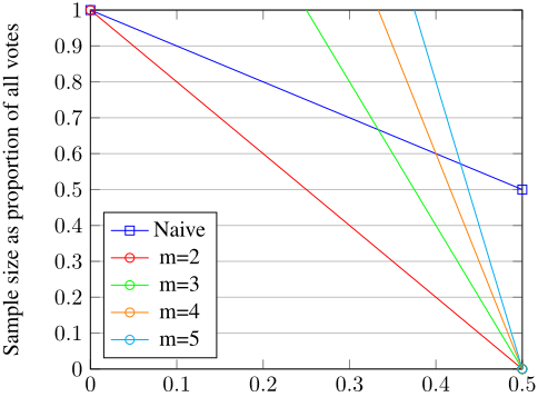
For any profile ⃗σ with margin of victory M(⃗σ), we can also develop upper bounds on the minimum sample size required for RCV to always be correct on any sufficiently large sample; these bounds are illustrated in Figure 1.
Proposition 2. For a profile ⃗σ consisting of n votes and m candidates, let x be the number of first choice votes for the RCV winner. All samples of size at least min(2(n - x) + 1, (m - 1)(n - 2M(⃗σ)) + 1) are guaranteed to return the correct winner.
Along the lines of Cary [2011], we may also derive upper and lower bounds on M(⃗σ) that depend on the sequence of eliminations taken by RCV.
Proposition 3. For a profile ⃗σ, M(⃗σ) ∈
where v(j) k for all j ∈ [1,m - k + 1] is the vote share for the j th most popular alternative in that round, and v(-1) k and v(-2) k are the vote shares of the alternatives that receive the fewest and second-fewest votes in round k, respectively.
7 In the full version, we describe another setup that, in mathematical simulations, does even worse than 1m! .
| RCV | Plurality | Borda | Harm. | Cope. | MM | Bucklin | Pl. Veto | Veto | ||
|---|---|---|---|---|---|---|---|---|---|---|
| M, ϕ = 0.5 | ACC MPW | 73.60 2.36e-2 | 68.97 1.05e-2 | 72.23 1.50e-2 | 70.37 1.07e-2 | 74.56 2.74e-2 | 74.43 2.67e-2 | 70.10 1.03e-2 | 97.46 8.76e-1 | 38.63 2.59e-5 |
| M, ϕ = 0.75 | ACC MPW | 44.15 6.83e-3 | 41.44 4.26e-3 | 46.70 8.60e-3 | 43.86 5.88e-3 | 45.96 7.46e-3 | 44.69 7.75e-3 | 43.30 5.26e-3 | 78.18 9.53e-1 | 33.49 9.98e-4 |
| Urn, α = 0.05 | ACC MPW | 40.13 1.48e-1 | 39.50 1.52e-1 | 38.56 1.12e-1 | 39.00 1.20e-1 | 39.34 1.33e-1 | 39.21 1.37e-1 | 37.30 1.24e-1 | 28.86 4.25e-2 | 24.71 3.13e-2 |
| Conitzer SPOC | ACC MPW | 27.91 1.11e-1 | 27.18 1.22e-1 | 27.74 1.14e-1 | 27.81 1.17e-1 | 27.50 9.88e-2 | 26.75 1.02e-1 | 26.67 1.10e-1 | 25.18 1.13e-1 | 23.25 1.12e-1 |
| Walsh SP | ACC MPW | 55.44 8.40e-2 | 46.67 1.92e-2 | 65.73 3.55e-1 | 56.53 7.13e-2 | 61.13 2.13e-1 | 61.53 2.13e-1 | 47.60 1.83e-2 | 43.94 2.48e-2 | 32.86 1.48e-3 |
| 3D Cube | ACC MPW | 47.64 1.09e-1 | 41.84 4.06e-2 | 56.38 3.04e-1 | 48.67 9.79e-2 | 51.72 1.67e-1 | 52.61 1.67e-1 | 47.35 7.61e-2 | 35.60 2.03e-2 | 37.60 1.81e-2 |
| 5D Sphere | ACC MPW | 31.08 1.31e-1 | 32.19 1.58e-1 | 27.99 8.70e-2 | 30.10 1.36e-1 | 28.81 9.61e-2 | 28.91 1.02e-1 | 29.11 1.15e-1 | 26.38 1.15e-1 | 17.11 6.10e-2 |
| RCV | Plurality | Borda | Harm. | Cope. | MM | Bucklin | Pl. Veto | Veto | ||
|---|---|---|---|---|---|---|---|---|---|---|
| M, ϕ = 0.5 | ACC MPW | 99.49 1.47e-1 | 98.50 1.31e-1 | 99.09 1.34e-1 | 99.06 1.38e-1 | 99.32 1.46e-1 | 99.31 1.46e-1 | 79.11 3.53e-3 | 1.000 1.52e-1 | 77.98 1.76e-3 |
| M, ϕ = 0.75 | ACC MPW | 82.30 1.50e-1 | 75.00 2.15e-2 | 79.64 1.20e-1 | 79.41 6.38e-2 | 83.01 1.54e-1 | 82.33 1.73e-1 | 69.85 1.23e-2 | 88.00 3.02e-1 | 62.25 2.74e-3 |
| Urn, α = 0.05 | ACC MPW | 70.85 2.73e-1 | 64.05 7.34e-2 | 63.02 1.03e-1 | 69.64 1.65e-1 | 66.65 1.67e-1 | 69.04 2.09e-1 | 45.57 9.43e-3 | 16.07 4.88e-5 | 33.42 7.97e-4 |
| Conitzer SPOC | ACC MPW | 49.46 2.17e-1 | 44.92 1.49e-1 | 44.08 1.42e-1 | 47.31 1.92e-1 | 43.11 1.32e-1 | 42.64 1.21e-1 | 29.48 1.72e-2 | 19.00 8.06e-3 | 29.92 2.15e-2 |
| Walsh SP | ACC MPW | 83.55 7.62e-2 | 79.78 4.16e-2 | 88.01 2.22e-1 | 86.17 2.11e-1 | 85.84 2.24e-1 | 87.87 2.26e-1 | 53.33 2.78e-4 | 3.770 8.95e-8 | 33.16 6.89e-6 |
| 3D Cube | ACC MPW | 77.78 2.16e-1 | 60.42 1.14e-2 | 74.82 1.49e-1 | 74.48 1.49e-1 | 75.16 2.20e-1 | 77.57 2.34e-1 | 66.05 1.90e-2 | 23.22 5.40e-6 | 53.99 2.49e-3 |
| 5D Sphere | ACC MPW | 82.15 2.40e-1 | 74.15 3.10e-1 | 81.43 4.11e-2 | 82.57 2.68e-1 | 82.52 5.67e-2 | 82.95 6.64e-2 | 72.38 1.35e-2 | 25.95 3.69e-3 | 10.41 1.30e-3 |
5 Experiments
In our experiments, we explore two main questions on a mix of synthetic elections generated from statistical cultures in the map of elections [Szufa et al., 2020; Boehmer et al., 2021] and real-world election data sourced from PrefLib [Mattei and Walsh, 2013] and the Harvard Dataverse [Harvard, 2020]. First, on synthetic elections, we examine the prediction accuracy of various voting rules when predicting the RCV winner on uniform samples of varying sizes. Second, on real-world elections, we examine the accuracy with which the RCV winner can be correctly predicted by each of the voting rules we consider, as well as two additional "ensemble" rules informed by results on the map of elections. Our code is available at https://github.com/miceland2/STV sampling.
5.1 Synthetic Elections
Informed by prior work on the map of elections, we use the mapel Python library to generate votes from the diverse set of statistical cultures included in the original map. These include the Mallows model (with dispersion parameter ϕ ∈
{0.001, 0.01, 0.05, 0.1, 0.25, 0.5, 0.75, 0.95, 0.99, 0.999}), Polya-Eggenberger urn models (with α ∈ {0.01, 0.02, 0.05, 0.1, 0.2, 0.5}), the Conitzer and Walsh single-peaked models, the Conitzer single-peaked on a circle (SPOC) model, singlecrossing models, the Impartial Culture model, 1D, 2D, 3D, 5D, 10D, and 20D hypercube models, and finally 2D, 3D, and 5D hypersphere models. In the interest of space, for further discussion of the specific statistical cultures in these models, see Section 2.2 in [Szufa et al., 2020].
In our experiments, we vary the sample size from 10% to 100% in steps of 10%, with the addition of a 5% sample size; omitted results can be found in the full version.
In Tables 1 and 2, we present the average prediction accuracy ("ACC") of each of our nine voting rules when predicting the RCV winner for profiles generated according to the statistical cultures we consider for samples consisting of 5% and 50% of the voters, respectively. The average prediction accuracy is taken over 100 samples on each of 100 different profiles generated according to the statistical cultures in consideration. These profiles each consist of 100 votes over 5
Margin of victory as proportion of all votes
Figure 1: Bounds on the minimum sample size needed to ensure that evaluating RCV on any sample will identify the correct winner. For each m, running RCV with any sample size above the corresponding line is guaranteed to return the correct winner.
alternatives, which is roughly the average number of candidates over all our real-world data.
For each statistical culture, we also treat each voting rule as an expert and learn normalized weights for each voting rule via the classic multiplicative weights ("MPW") algorithm [Littlestone and Warmuth, 1994; Arora et al., 2012].
Overall, we find that RCV exhibits uneven performance across different statistical vote cultures, but its accuracy increases with sample size. Plurality Veto is unexpectedly accurate for Mallows models, as evinced by its remarkably high MPW score in these settings. On the whole, we observe that more "centered" distributions like Mallows are generally easier to predict than other families, most likely due to RCV's sensitivity to the order of eliminations in scenarios without a clear majority winner.
5.2 Real-World Elections
One of our main empirical questions is whether we can leverage results from synthetic vote profiles to achieve greater prediction accuracy on real-world elections. To this end, we build two ensemble methods that leverage the pseudodistance metric underlying the map of elections in order to predict the RCV winner of real-world elections.
The central idea behind these ensemble methods is to use good predictors of RCV on "nearby" elections on the map of elections in order to predict RCV outcomes on real-world data. Given a sample s, both ensemble methods first identify the closest statistical culture according to positionwise distance as defined in Section 3.2 in [Szufa et al., 2020]. We call the closest statistical culture C, and use our empirical results on C to create scores for each alternative. Throughout, let R represent the set of rules we define in Section 2.1.
The first ensemble method, which we term "Summation," uses our experiments on synthetic data and adds accf(C), which we define as the empirical accuracy of rule f predicting RCV on culture C, to the score of the winner f(s) for each rule f ∈ R. The alternative with the highest overall score after this process is the Summation winner.
The second ensemble method, which we call "MPW," selects a predictive rule to use according to a probability distribution based on the normalized weights learned on C through the multiplicative weights process. The alternative returned by the predictive rule is the MPWwinner.
We run experiments to measure the performance of the nine rules in Section 2.1, as well as these two ensemble rules, on a total of 12 collections of different real-world elections from PrefLib [Mattei and Walsh, 2013] and Harvard Dataverse [Harvard, 2020], amounting to a total of 275 individual elections. Each collection consists of between 8 and 46 separate elections, each of which contain between 143 and 39,401 votes on 2 to 15 candidates. Full descriptions can be found in the full version.
Preprocessing
For each dataset in the Harvard database, we take all available profiles of the locality and government position. We exclude elections that consist of a single candidate. For each profile, we (1) discard blank rows, (2) remove table cells labeled "write-in," "overvote," or "skipped," and (3) keep only the higher-ranked position for each vote if the voter gave two or more rankings of the same alternatives. Generally, the final preprocessing step applied to less than 10% of all votes for each profile. In contrast, datasets from Preflib did not require the preprocessing steps described above.
All real-world elections give strict-order-incomplete rankings over the candidates, where unranked candidates in a given vote are assumed to be tied for last place. We complete each of these incomplete rankings using the same method proposed by Boehmer et al. [2021] in order to (1) run each of our voting rules without modifications or additional assumptions and (2) compute the positionwise distances between each real election and those from the map of elections using the mapel library. For each vote v that gives an incomplete ranking for their top t candidates, we first draw uniformly at random another vote that ranks at least the top (t + 1) candidates and agrees with v on the top t candidates, and we then extend v with this other vote's (t + 1)st -ranked candidate. If no such vote exists, we extend v with one of their unranked candidates uniformly at random. The process is repeated until all votes are strict-order complete.
Real-World Results
We present the average RCV sampling accuracies for each of our rules for three collections of elections in Figure 2. For each sample size (5%, 10%, 30%, 50%, 70%, and 100%) and each election, we estimate the sampling accuracy with 1,000 samples. The right-most column contains average accuracies for all elections in each group, and the other two columns show results from individual elections in each group. The center column contains plots that are more typical of the dataset, while those on the left are more extraneous and typically have lower bounds on the margin of victory.
We observe that, in contrast to the theoretical results and results on synthetic data, RCV is on average one of the best predictors of itself even on low sample sizes. While this does not mean that RCV is the best predictor of itself on every individual election, on average, this trend persists over all our real-world data. Only among the Glasgow City Council elections, though, is RCV decisively the best predictor. Summation performs almost as well as RCV on average. This is likely because the ensemble rules tend to agree with RCV on high sample sizes for all the real-world data we considered, whereas other voting rules sometimes diverged from the RCV winner as sample size increases. The Condorcet-consistent rules, namely Copeland and Minimax, are also among the best predictors of RCV and only rarely diverge from the true winner. On the other hand, MPW often suffers from poor performance on low sample sizes before catching up at higher sample sizes. This is because, as seen in Tables 1 and 2, Plurality Veto has a very high weight in small samples for Mallows elections; its weight decreases as sample size increases. However, Plurality Veto often does poorly in predicting the overall RCV winner in practice. Although on some profiles, such as in the top-left and bottom-left of Figure 2, Plurality Veto is an exceptional predictor of RCV even on 5% sample sizes, such profiles are not common, and Plurality Veto often does not increase in accuracy as sample size increases.
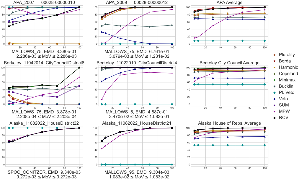
We also note that, in direct contrast to our worst-case results, the average predictive performance of RCV increases with sample size, corroborating prior observations that realworld elections are far from the worst-case profiles we study [Boehmer and Schaar, 2023].
Finally, we conclude that the positionwise distance is limited in its ability to extrapolate sampling behavior from one election to a nearby election in terms of positionwise distance. The most obvious evidence comes from the disparity in performance of Plurality Veto between the synthetic Mallows profiles and the real-world elections. As seen in Figure 2, Plurality Veto is by far the worst, on average, at predicting RCV for all three datasets, yet most of their profiles are closest to one of the Mallows cultures. This disparity in performance can be explained by the fact that a given positionwise frequency matrix can map to several different profiles, as explored in [Boehmer et al., 2023].
6 Discussion
This paper presents a theoretical and empirical exploration of using RCV on samples to predict the outcome of applying RCV on the entire election. We establish that, while RCV exhibits bad worst-case theoretical accuracy, it is generally the most trustworthy predictor of itself in practice.
As for future work, there are two main avenues to pursue. With respect to theoretical results, it would be interesting to fully characterize the conjectured monotonicity of the worst-case prediction accuracy of RCV. We present some initial results toward this goal in the full version. We also will study average-case predictability of RCV on samples instead of worst-case predictability.
Acknowledgments
The authors would like to thank David McCune for his helpful comments on STV and for pointing us to the Harvard Dataverse, as well as anonymous AAAI reviewers for their thoughtful suggestions.
@inproceedings{ijcai2024p314,
  title     = {Sampling Winners in Ranked Choice Voting},
  author    = {Iceland, Matthew and Kahng, Anson and Saber, Joseph},
  booktitle = {Proceedings of the Thirty-Third International Joint Conference on
               Artificial Intelligence, {IJCAI-24}},
  publisher = {International Joint Conferences on Artificial Intelligence Organization},
  editor    = {Kate Larson},
  pages     = {2834--2841},
  year      = {2024},
  month     = {8},
  note      = {Main Track},
  doi       = {10.24963/ijcai.2024/314},
  url       = {https://doi.org/10.24963/ijcai.2024/314},
}
TY - CPAPER TI - Sampling Winners in Ranked Choice Voting AU - Iceland, Matthew AU - Kahng, Anson AU - Saber, Joseph T2 - Proceedings of the Thirty-Third International Joint Conference on Artificial Intelligence, IJCAI-24 PB - International Joint Conferences on Artificial Intelligence Organization PY - 2024 SP - 2834 EP - 2841 DO - 10.24963/ijcai.2024/314 UR - https://doi.org/10.24963/ijcai.2024/314 ER -Copied
Machine-readable versions of this paper, for tools and AI agents:





