Putting a Compass on the Map of Elections

1 Introduction

Experiments are gaining increasing attention in the computational social choice literature. While such studies often give insights that would be very difficult to obtain otherwise, they are not easy to design. For example, if we wanted to evaluate the running time of a certain algorithm for computing election winners, what data should we run it on? To answer such questions, we need to understand the space of possible elections. This includes knowing, e.g., what elections arise in practice, what elections are generated from standard election models, what makes elections difficult for our algorithm, and so on. In this paper we continue the quest for understanding the space of election by means of analyzing their distances, as initiated by Szufa et al. [2020].

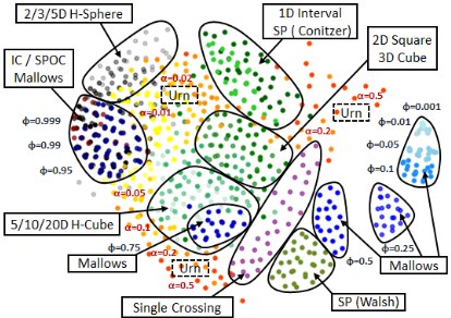
Specifically, Szufa et al. [2020] proposed a technique for visualizing sets of ordinal elections-i.e., elections where each voter ranks the candidates from the most to the least appealing one-based on given distances between them. They have applied this technique to 800 elections coming from various statistical cultures, ranging from the classic urn and Mallows models to various types of restricted domains, and they obtained a map of elections, where elections with similar properties are grouped together (see Figure 1; each dot represents a single election and, generally, the closer two elections are in the picture, the smaller is their distance). Indeed, we see that elections from the same statistical cultures, represented with the same color, are nicely grouped together; Szufa et al. [2020] have also shown other evidence that nearby elections are closely related. 1 Yet, the map has two major drawbacks. First, while similar elections are plotted next to each other, there is no clear meaning to absolute positions on the map. Second, the map regards statistical cultures only and it is not obvious where real-life elections-such as those stored in PrefLib [Mattei and Walsh, 2013]-would lie on the map. Our goal is to address both these issues.

We start by looking more closely at the distance metric for elections that Szufa et al. [2020] used. The idea is that given an election with m candidates, one computes an m×m frequency matrix which specifies what fraction of the voters ranks each candidate in each position (such matrices are bistochastic, i.e., their entries are nonnegative and each column and each row sums up to one). Measuring the distance between two elections boils down to computing their frequency matrices and summing up the earth mover's distances between their columns, where columns are reordered to min-

1 The map in the figure regards elections with 10 candidates and 100 voters, whereas Szufa et al. [2020] focused on the case of 100 candidates and 100 voters. Nonetheless, they also provided such smaller datasets and we focus on them because we want to compare them to real-life elections, which typically have few candidates.

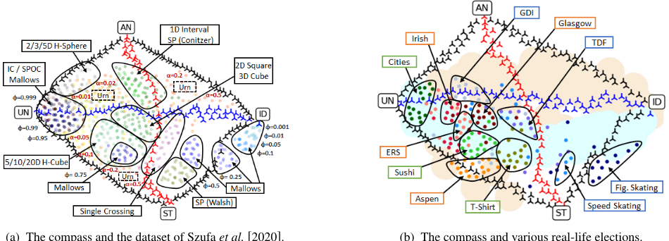
• (a) The compass and the dataset of Szufa et al. [2020].
• (b) The compass and various real-life elections.

Figure 2: Maps of elections for the 10x100 dataset of Szufa et al. [2020] (on the left) and some real-life elections (on the right). The maps include the compass matrices and their connecting paths (shown in black, red, and blue). To highlight the paths, the dots corresponding to the elections of Szufa et al. [2020] (in the left figure) are shown in lighter colors than in Figure 1. On the right, the pale blue area is where Mallows elections end up (for various φ parameters) and the pale orange area is where urn elections end up (for various α parameters).

imize the distance (see Section 2 for definitions); Szufa et al. [2020] call this distance positionwise. Using frequency matrices makes it possible to compare elections with different numbers of voters, and reordering the columns ensures that candidate names are irrelevant (as suggested for such settings by Faliszewski et al. [2019]).

Our first result is an algorithm that, given a bistochastic matrix and a number n, finds some election with n voters whose frequency matrix is (nearly) identical to the one from the input (achieving perfect accuracy is not always possible, but our algorithm achieves the best result one may, in general, hope for). As a consequence, instead of considering elections, we may directly look at the space of bistochastic matrices, which simplifies many discussions. Consequently, we often speak of matrices and elections interchangeably.

Next, we form what we call a compass. The idea is to pick matrices that, on the one hand, are far away from each other, and, on the other hand, have natural interpretations. Specifically, we consider the following four "extreme" matrices, corresponding to four types of (dis)agreement among the voters:

1. The identity matrix, ID, modelling perfect agreement (all voters have the same preference order).
2. The uniformity matrix, UN, modelling lack of agreement (each candidate takes each position equally often).
3. The stratification matrix, ST, modelling partial agreement (voters agree that half of the candidates are better than the other half, but lack agreement on anything else).
4. The antagonismmatrix, AN, modelling conflict (half of the voters have opposite preferences to the other half).

For each two of these "compass" matrices, we also consider a spectrum of their convex combinations ("paths" between the matrices). In visualizations, these paths appear as a parallelogram-like shape with corresponding "diagonals"; see, e.g., Figure 2a, where we apply the compass method to the dataset from Figure 1 (the black, blue, and red points are certain convex combinations of the corresponding endpoints, which are the compass matrices). The remainder of the paper largely consists of explaining why we get what we see here.

The compass allows us to make a number of observations. For example, in Figure 2a we see that 1D Interval elections are closer to the antagonism matrix, whereas higherdimensional hypercube elections are closer to the stratification one. This is intriguing as, on a formal level, these two kinds of elections are very similar. Figure 2b, which shows a map of real-life elections (some from PrefLib and some new ones) is even more striking. Most of the real-life elections (including all political ones) end up in one "quadrant" of the parallelogram, and essentially all elections end up in the vicinity of some Mallows elections (the pale blue area is where Mallows elections end up, depending on the parameter of the model; the pale orange area is where urn elections end up). So, if one were to run experiments with a single statistical culture, the Mallows model might be a wise choice.

Yet, we find that seemingly natural ways of sampling Mallows elections (e.g., by choosing the Mallows parameter uniformly at random, or using a fixed parameter for different numbers of candidates), which are used in many research papers, are biased. We propose a normalization and argue, both theoretically and by considering the compass, that it produces more balanced results. In other words, we recommend using the Mallows model, but in conjunction with our normalization.

We provide details missing from this paper in its full version, available as a technical report [Boehmer et al., 2021].

2 Preliminaries

Given an integer t, we write [t] to denote the set {1, . . . , t}. By R+ we mean the set of nonnegative real numbers. Given a vector x = (x1, . . . , xm), we interpret it as an m× 1 matrix, i.e., we use column vectors. For a matrix X, we write xi,j to refer to the entry in its i-th row and j-th column.

Elections. An election E is a pair (C, V ), where C = {c1, . . . , cm} is a set of candidates and V = (v1, . . . , vn) is a collection of voters. Each voter v ∈ V has a preference order ≻v, which ranks the candidates from the most to the least desirable one according to v. If v prefers candidate a to candidate b, then we write v : a ≻ b, and we extend this notation to more candidates in a natural way. For a voter v and a candidate c, we write posv(c) to denote the position on which v ranks c (the top-ranked candidate has position 1, the next one has position 2, and so on). We refer to both the voters and their preference orders as the votes. The intended meaning will always be clear from the context.

Position and frequency matrices. Let E = (C, V ) be an election, where C = {c1, . . . , cm} and V = (v1, . . . , vn). For a candidate c ∈ C and position i ∈ [m], we write #posE(c, i) to denote the number of voters in election E that rank c on position i. By #posE(c) we mean the vector:

The position matrix for election E, denoted #pos(E), is the m×mmatrix that has vectors #posE(c1), . . . ,#posE(cm) as its columns. We also consider vote frequencies rather than absolute counts. To this end, for a candidate c and a position i ∈ [m], let #freqE(c, i) = #posE (c,i)/n, let vector #freqE(c) = (#freqE(c, 1), . . . ,#freqE(c,m)), and let the frequency matrix for election E, denoted #freq(E), consist of columns #freqE(c1), . . . ,#freqE(cm). Note that in each position matrix, each row and each column sums up to the number of voters in the election. Similarly, in each frequency matrix, the rows and columns sum up to one (such matrices are called bistochastic).

Example 1. Let E = (C, V ) be an election, where C = {a, b, c}, V = (v1, . . . , v6), and the preference orders are v1 : a ≻ b ≻ c, v2 : a ≻ b ≻ c, v3 : a ≻ b ≻ c, v4 : b ≻ a ≻ c, v5 : c ≻ a ≻ b, v6 : c ≻ a ≻ b. The position and frequency matrices for this election are:

Earthmover's distance (EMD). Let x = (x1, . . . , xt) and y = (y1, . . . , yt) be two vectors from Rt+, whose entries sum up to 1. The earth mover's distance between x and y, denoted EMD(x, y), is defined as the lowest total cost of operations that transform vector x into vector y, where each operation is of the form "subtract δ from position i and add δ to position j" and costs δ · |i - j|. Such an operation is legal if the current value at position i is at least δ. EMD(x, y) can be computed in polynomial time using a greedy algorithm.

Positionwise distance. Let E = (C, V ) and F = (D,U) be two elections with m candidates each (we do not require that |V | = |U|). The positionwise distance between E and F, denoted POS(E, F), is defined in terms of frequency matrices #freq(E) = (e1, . . . , em) and #freq(F ) = (f1, . . . , fm) as follows [Szufa et al., 2020]:

where Sm is the permutation group on m elements. In other words, the positionwise distance is the sum of the earth mover's distances between the frequency vectors of the candidates from the two elections, matched optimally according to σ. The positionwise distance is invariant to renaming the candidates and reordering the voters.

Statistical cultures. We define the following three statistical cultures, i.e., models of generating random elections: 2

Impartial culture Under the Impartial Culture (IC) model, we sample all votes uniformly at random.

P´olya-Eggenberger urn model [Berg, 1985] The urn model uses a nonnegative parameter α, which gives the level of correlation between the votes (this parameterization is due to McCabe-Dansted and Slinko [2006]). To generate an election with m candidates, we start with an urn containing one copy of each possible preference order and generate the votes iteratively: In each step we uniformly at random draw an order from the urn (this is the voter's preference order) and return it to the urn together with αm! copies. For α = 0 we obtain the IC model.

Mallows model [Mallows, 1957] The Mallows model uses parameter φ ∈ [0, 1] and a central preference order v. Each vote is generated randomly and independently. The probability of generating preference order u is proportional to φκ(v,u) , where κ(v, u) is the swap distance between u and v (i.e., the minimum number of swaps of adjacent candidates needed to transform u into v).

Maps of elections. Szufa et al. [2020] drew a map of elections by computing the positionwise distances between 800 elections drawn from various statistical cultures and visualizing them using the force-directed algorithm of Fruchterman and Reingold [1991]. They focused on elections with 100 candidates and 100 voters, but also generated smaller datasets, available on their website. We consider their dataset with 10 candidates and 100 voters (see Figure 1 for its map). We use the same algorithm as they do for our visualizations, except that for each two elections we set their attraction coefficient to be the square of their positionwise distance (and not the distance itself, as done by Szufa et al.; this groups similar elections more tightly and gives more visually appealing results for elections with few candidates). We stress that the maps that both we and Szufa et al. [2020] provide are helpful tools to illustrate the distances between particular (families of) elections, but are certainly not perfect. For example, since the visualization algorithm is randomized, we can get slightly different maps for each run of the algorithm. The visualizations also depend on the exact composition of the set of depicted elections. Thus, whenever we say that some two elections are close to each other, we mean that their positionwise distance is small. While this is typically reflected by these two elections being close on the map, on its own, closeness on the map does not suffice for such a claim.

2 Sometimes, we refer to other statistical cultures used by Szufa et al. [2020]. We do not define them formally here, but we attempt to make our discussions intuitively clear.

3 Recovering Elections fromMatrices

Throughout this paper we often deal with frequency matrices of elections. While computing a frequency matrix of an election is straightforward, the reverse direction is less clear.

We first note that each m×m position matrix has a corresponding m-candidate election with at most m2 - 2m + 2 distinct preference orders.

Proposition 1 (Leep and Myerson [1999]). Given an m× m position matrix X, one can compute in O(m4.5 ) time an election E with at most m2 - 2m + 2 different votes, such that #pos(E) = X.

Next, we consider recovering elections based on frequency matrices. Given an m×m bistochastic matrix X and a number n of voters, we would like to find an election E with position matrix nX. This may be impossible as nX may have fractional entries, but we can get very close to this goal. The next proposition justifies speaking of elections and frequency matrices interchangeably.

Proposition 2. Given an m × m bistochastic matrix X and an integer n, one can compute in polynomial time an election E with n voters whose position matrix P satisfies |nxi,j - pi,j| ≤ 1 for each i, j ∈ [m] and, under this condition, minimizes the value ∑1≤i,j≤m |nxi,j - pi,j |.

4 Setting up the Compass

Our "compass" consists of two main components: Four matrices that occupy very different areas of the election space and represent different types of (dis)agreement among the voters, and six paths consisting of their convex combinations.

4.1 The Four Matrices

Below we define the four matrices and explain our choice.

Identity and uniformity. Our first two matrices are the identity matrix, IDm, with ones on the diagonal and zeros elsewhere, and the uniformity matrix, UNm, with each entry equal to 1/m. The identity matrix corresponds to elections where each voter has the same preference order, i.e., there is a common ordering of the candidates from the most to the least desirable one. In contrast, the uniformity matrix captures elections where each candidate is ranked on each position equally often, i.e., where, in aggregate, all the candidates are viewed as equally good. Uniformity elections are quite similar to the IC ones and, in the limit, indistinguishable from them (i.e., with sufficiently many voters, we would not see a difference between IC and UN; with fewer voters, IC elections are at some small distance from uniformity).

Stratification. The next matrix, stratification, is defined as follows (we assume that m is even):

Stratification matrices correspond to elections where the voters agree that half of the candidates are more desirable than the other half, but, in aggregate, are unable to distinguish between the qualities of the candidates in each group.

Antagonism. Let rIDm be thematrix obtained by reversing the order of the columns of the identity matrix IDm. We define the antagonism matrix, ANm, to be 1/2IDm + 1/2rIDm. Such matrices are generated, e.g., by elections where half of the voters rank the candidates in one order, and half of the voters rank them in the opposite one, so there is a clear conflict. In some sense, stratification and antagonism are based on similar premises. Under stratification, the group of candidates is partitioned into halves with different properties, whereas in antagonism the voters are partitioned. However, the nature of the partitioning is, naturally, quite different.

We chose the above matrices because they capture natural, intuitive phenomena and seem to occupy very different areas of the space of elections (although we are sure that other choices would be possible, too). Below we calculate the positionwise distances between our matrices.

Proposition 3. If m is divisible by 4, then it holds that:

1. POS(IDm,UNm) = 1 3 (m2 - 1),

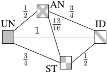
To normalize these distances, we divide them by D(m) = POS(IDm,UNm), which we suspect to be the largest positionwise distance between two matrices over m candidates. For each two matrices X and Y among our four, we let d(X, Y ) := limm→∞ POS(Xm,Ym)/D(m). A simple computation shows the following (see also Figure 3a; we sometimes omit the m subscript for clarity):

For small m, using ILPs, we verified that each compass matrix is almost as far away as possible from the others. Similarly, for each m ∈ {3, . . . , 7} we verified that IDm and UNm are the two most distant matrices under the positionwise distance. Indeed, we believe that ID and UN are the two most distant frequency matrices, i.e., they form the diameter of our space. However, showing this seems to be challenging.

4.2 Paths Between ElectionMatrices

Next, we consider convex combinations of frequency matrices. Given two such matrices, X and Y , and α ∈ [0, 1], one might expect that matrix Z = αX + (1 - α)Y would lie at distance (1 - α)POS(X, Y ) from X and at distance αPOS(X, Y ) from Y , so that we would have:

However, without further assumptions this is not necessarily the case. Indeed, if we take X = IDm and Y = rIDm, then 0.5X + 0.5Y = ANm and POS(X, Y ) = 0, but POS(X, 0.5X + 0.5Y ) = POS(ID,AN) > 0. Yet, if we arrange the two matrices X and Y so that their positionwise distance is achieved by the identity permutation of their column vectors, then their convex combination lies exactly between them.

• (c) Mallows elections (teal); φ chosen uniformly at random.

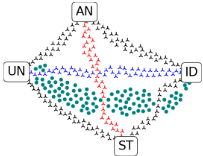
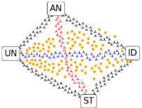
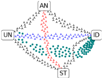
Figure 3: Visualization of our four matrices and the connecting paths. In Figure 3a we show the normalized distances between the four matrices, whereas in the remaining three pictures we show the matrices, the connecting paths, and, respectively, urn elections and Mallows elections (for two distributions of their parameter). These visualizations are for 20 candidates and 100 voters.

Proposition 4. Let X = (x1, . . . , xm) and Y = (y1, . . . ym) be two m×m frequency matrices such that:

Using Proposition 4, for each two compass matrices we can generate a sequence of matrices that form a path between them. For example, matrix 0.5ID+ 0.5UN is exactly at the same distance from ID and from UN. In Figure 2a we show a map of elections that (in addition to the dataset of Szufa et al. [2020]) contains our four compass matrices and for each two of them, a set of ⌈50·d(X, Y )⌉ matrices obtained as their convex combinations with values of α uniformly distributed in [0, 1]. For all other maps including the compass, the six paths were generated in the same way. The positionwise distances between any two of our four matrices are achieved by the identity permutation, as required by Proposition 4.

5 Applying the Compass

In this section, we apply our compass for a deeper understanding of the map of elections created by Szufa et al. [2020] and place some real-life elections on the map. We also consider where Mallows and urn elections land on the maps.

5.1 AMap of Statistical Cultures with a Compass

In Figure 2a, we show a map of the 800 elections provided by Szufa et al. [2020] in their 10x100 dataset, together with the compass. As expected, the uniformity matrix is close to the impartial culture elections, but still at some distance from them. Similarly, the identity matrix is very close to the Mallows elections with close-to-zero values of φ. Indeed, such elections consist of nearly identical votes.

The red path, linking AN and ST, roughly partitions the elections into those closer to UN and those closer to ID. The latter group consists mostly of Mallows and urn elections (with low φ or high α, respectively), but single-crossing and some single-peaked elections also make an appearance.

Analyzing the distances of elections to AN and ST, it is striking that 1D Interval elections lie closer to AN, while other hypercube elections lie closer to ST, even though, formally, they are similar. It is also intriguing that single-peaked elections generated according to the Walsh model [Walsh,

2015] are closer to ST, whereas those from the Conitzer model [Conitzer, 2009] (which are very similar to the 1D Interval ones) are closer to AN. 3 A brief explanation for readers familiar with single-peaked elections is as follows. In the Conitzer model, given a societal axis (i.e., an underlying order of the candidates, e.g., from left to right in the political spectrum), we generate a vote by choosing a top-ranked candidate uniformly at random and extending the vote with candidates to the left and to the right (on the axis) with equal probability. So, by choosing close-to-extreme candidates from different sides of the axis as top-ranked, we generate close-to-opposite preference orders with fairly high probability. Under the Walsh model, we choose each single-peaked preference order uniformly at random. There are few such preference orders with extreme candidates ranked highly, but many with the center ones on top. This leads to stratification.

5.2 Urn andMallows Elections

Our next goal is to place "paths" of urn and Mallows elections on the map. In both cases it requires some care. Recall that the urn model has parameter α, which takes values between 0 and ∞. To generate an urn election, we choose α according to the Gamma distribution with shape parameter k = 0.8 and scale parameter θ = 1 (this ensures that about half of the urn elections are closer to UN than to ID; see Figure 3b).

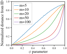
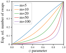
Regarding the Mallows model, we have a parameter φ that takes values between 0 and 1, where 0 leads to generating ID elections and 1 leads to generating IC ones. It is thus intuitive to choose φ uniformly at random from the [0, 1] interval. Yet, as seen in Figure 3c, doing so places elections quite unevenly on the map. Similarly, for different numbers of candidates the same value of φ leads to choosing elections at different distances from ID (see the left part of Figure 4). Thus we seek a new parameterization of the Mallows model.

Normalizing Mallows. Consider a setting with m candidates. For φ ∈ [0, 1], let expswaps(m, φ) be the expected swap distance between an m-candidate vote generated using the Mallows model with parameter φ and the center vote. We define the relative expected number of swaps as relswaps(m, φ) = expswaps(m,φ) m(m-1)/2 (see the right part of Figure 4 for plots of this value). In our approach, we choose a value rel-φ ∈ [0, 1] as a parameter, find a φ such that relswaps(m, φ) = rel-φ, and draw an election from the Mallows model using this φ (see the full paper for details). Working on rel-φ instead of φ not only allows for an intuitive and natural interpretation of the parameter as the relative expected number of swaps in each vote (or the normalized distance from ID), but also for obtaining comparable elections for different numbers of candidates. In Figures 3c and 3d we visualize Mallows elections generated with φ ∈ [0, 1] and relφ ∈ [0, 0.5] chosen uniformly at random, respectively (we use rel-φ ≤ 0.5 because for larger values one obtains analogous elections, but reversed; e.g., both rel-φ = 0 and rel-φ = 1 lead to identity elections). Figure 3d shows a far more balanced distribution of points.

3 The average distance of Walsh elections to ST is about half of their distance to AN; for Conitzer elections this relation is reversed.

Importance of the new normalization. The new parameterization of Mallows seems to be important. The Mallows model is often used in experiments and-in light of our findings-using a fixed φ for different numbers of candidates or drawing φ from a distribution independent of the number of candidates, may be questionable. Yet, this is not uncommon, as witnessed, e.g., in the works of Betzler et al. [2014], Goldsmith et al. [2014], Skowron et al. [2015], Bachrach et al. [2016], Garg et al. [2019], and in a number of other papers. We mention these works as examples only; their authors designed their experiments as best practice suggested at the time and we do not challenge their high-level conclusions. Our point is that given the current evidence, they might prefer to design their experiments a bit differently.

5.3 Real-Life Elections on the Map

Let us now consider where real-life elections appear on the map. We start by describing the datasets that we use (mostly from PrefLib, due to Mattei and Walsh [2013]). See the full paper for details on how the data was selected and preprocessed. In particular, we converted partial preference orders to complete ones using a simplified variant of the approach proposed by Doucette [2016]. Whenever we speak of real-life elections in this section, we mean elections from our datasets.

We chose eleven real-life datasets, where each belongs to one of three groups. The first group contains political elections: city council elections from Glasgow and Aspen ([O'Neill, 2013]), elections from North Dublin, Meath (Irish), and elections held by non-profit organizations, trade unions, and professional organizations (ERS). The second group consists of sport elections: Tour de France (TDF), Giro d'Italia (GDI), speed skating, and figure skating (the former three dataset are due to us). The last group consists of surveys: preferences over Sushi, T-Shirt designs, and costs of living and population in different cities ([Caragiannis et al., 2019]). For TDF and GDI, each race is a vote, and each season is an election. For speed skating, each lap is a vote, and each competition is an election. For figure skating, each judge's opinion is a vote, and each competition is an election.

In Figure 2b we show a map of these real-life elections along with the compass, Mallows, and Urn elections. For readability we present Mallows and Urn elections as large, pale-colored areas. Not all real-life elections form clear clusters, hence the labels refer to largest compact groupings.

While the map is not a perfect representation of distances among elections, analyzing it leads to many conclusions. Most strikingly, real-life elections occupy a very limited area of the map; this is especially true for political elections and surveys. Except for several sport elections, all elections are closer to UN than to ID (strictly speaking, this is true for 142 elections out of 165), and none of the real-life elections falls in the top-right part of the map (in the visualization). Another observation is that Mallows elections go right through the real-life elections, while Urn elections are on average far away. This means that for most real-life elections there exists a parameter φ such that elections generated according to the Mallows model with that parameter are relatively close (in particular, we suggest using rel-φ ∈ [0.36, 0.39] to capture political elections; see the full paper for more details).

Most of the political elections lie close to one another and are located next to Mallows elections and high-dimensional hypercube ones. Sport elections are spread over a larger part of the map and, with the exception of GDI, are shifted toward ID. As to the surveys, the City survey is basically equivalent to a sample from IC. The Sushi survey is similar to political elections. The T-shirt survey is shifted toward stratification.

6 Summary

We have provided a way to interpret locations on the map of elections of Szufa et al. [2020]. We have also shown where real-life elections end up on this map, which lead to a number of observations regarding both synthetic and real-life elections. In doing so, we identified and fixed a certain flaw in a typical way of sampling Mallows elections. It is important to confirm our experimental observations theoretically. Perhaps the most pressing such issue is to verify if identity and uniformity indeed are the two most distant frequency matrices.

Acknowledgments

Niclas Boehmer was supported by the DFG project MaMu (NI 369/19). This project has received funding from the European Research Council (ERC) under the European Union's Horizon 2020 research and innovation programme (grant agreement No 101002854).