
Polynomial Time Presolve Algorithms for Rotation-Based Models Solving the Robust Stable Matching Problem
Proceedings of the Thirty-Third International Joint Conference on Artificial Intelligence. Main Track. Pages 2860-2867.
https://doi.org/10.24963/ijcai.2024/317
Keywords
- Constraint Satisfaction and Optimization: CSO: Modeling
- Knowledge Representation and Reasoning: KRR: Preference modelling and preference-based reasoning
- Game Theory and Economic Paradigms: GTEP: Computational social choice
- AI Ethics, Trust, Fairness: ETF: Safety and robustness
Abstract
The Robust Stable Matching (RSM) problem involves finding a stable matching that allows getting another stable matching within a minimum number of changes when a pair becomes forbidden. It has been shown that such a problem is NP-Hard. In this paper, we enrich the mathematical model for the RSM problem based on new theoretical properties. We derive from these properties new polynomial time pre-solving algorithms which both reduce the search space and speed up the exploration. We also extend our results to the instances of the Many-to-Many problem and give its corresponding constraint programming (CP) model. We show how the use of our algorithms improve the state-of-the-art results and make it possible to obtain proofs of optimality on large instances via the CP model.
- [Baıou and Balinski, 2000] Mourad Baıou and Michel Balinski. Many-to-many matching: stable polyandrous polygamy (or polygamous polyandry). Discrete Applied Mathematics, 101(1-3):1-12, 2000.
- [Bansal et al., 2007] Vipul Bansal, Aseem Agrawal, and Varun S Malhotra. Polynomial time algorithm for an opti- mal stable assignment with multiple partners. Theoretical Computer Science, 379(3):317-328, 2007.
- [Biró and McDermid, 2008] Peter Biró and Eric McDermid. Three-sided stable matchings with cyclic preferences and the kidney exchange problem. In Proceedings of COM- SOC: 2nd International Workshop on Computational So- cial Choice, pages 97-108, 2008.
- [Cheng, 2010] Christine T Cheng. Understanding the gener- alized median stable matchings. Algorithmica, 58:34-51, 2010.
- [Chisca et al., 2016] Danuta Chisca, Mohamed Siala, Gilles Simonin, and Barry O'Sullivan. A cp-based approach for popular matching. In Proceedings of the AAAI Conference on Artificial Intelligence, volume 30, 2016.
- [Cseh et al., 2021] Ágnes Cseh, Guillaume Escamocher, Begüm Genc ¸, and Luis Quesada. A collection of con- straint programming models for the three-dimensional sta- ble matching problem with cyclic preferences. 2021.
- [Dasgupta and Maskin, 2008] Partha Dasgupta and Eric Maskin. On the robustness of majority rule. Journal of the European Economic Association, 6(5):949-973, 2008.
- [Eirinakis et al., 2012] Pavlos Eirinakis, Dimitrios Magos, Ioannis Mourtos, and Panayiotis Miliotis. Finding all stable pairs and solutions to the many-to-many stable matching problem. INFORMS Journal on Computing, 24(2):245-259, 2012.
- [Gale and Shapley, 1962] David Gale and Lloyd S Shapley. College admissions and the stability of marriage. The American Mathematical Monthly, 69(1):9-15, 1962.
- [Genc et al., 2017] Begum Genc, Mohamed Siala, Gilles Si- monin, and Barry O'Sullivan. Finding robust solutions to stable marriage. In Proceedings of the 26th Interna- tional Joint Conference on Artificial Intelligence, pages 631-637, 2017. IJCAI
- [Genc et al., 2019] Begum Genc, Mohamed Siala, Gilles Si- monin, and Barry O'Sullivan. Complexity study for the ro- bust stable marriage problem. Theoretical Computer Sci- ence, 775:76-92, 2019.
- [Genc, 2019] Begum Genc. An approach to robustness in stable marriage and stable roommates problems. PhD the- sis, University College Cork, 2019.
- [Gervet, 1995] Carmen Gervet. Set Intervals in Constraint Logic Programming: Definition and implementation of a language. PhD thesis, Université de Franche Comté Besanc ¸on, 1995.
- [Gervet, 1997] Carmen Gervet. Interval propagation to rea- son about sets: Definition and implementation of a practi- cal language. Constraints, 1:191-244, 1997.
- [Ginsberg et al., 1998] Matthew L Ginsberg, Andrew J Parkes, and Amitabha Roy. Supermodels and robustness. In AAAI/IAAI, pages 334-339, 1998.
- [Gusfield and Irving, 1989] Dan Gusfield and Robert W Irv- ing. The stable marriage problem: structure and algo- rithms. MIT press, 1989.
- [Hebrard et al., 2004] Emmanuel Hebrard, Brahim Hnich, and Toby Walsh. Super solutions in constraint program- ming. In International conference on integration of ar- tificial intelligence (AI) and operations research (OR) techniques in constraint programming, pages 157-172. Springer, 2004.
- [Irving and Leather, 1986] Robert W Irving and Paul Leather. The complexity of counting stable marriages. SIAM Journal on Computing, 15(3):655-667, 1986.
- [Jacobovic, 2016] Royi Jacobovic. Perturbation robust stable matching. arXiv e-prints, pages arXiv-1612, 2016.
- [Mai and Vazirani, 2018] Tung Mai and Vijay V. Vazirani. Finding Stable Matchings That Are Robust to Errors in the Input. In Yossi Azar, Hannah Bast, and Grzegorz Herman, editors, 26th Annual European Symposium on Algorithms (ESA 2018), volume 112 of Leibniz International Proceed- ings in Informatics (LIPIcs), pages 60:1-60:11, Dagstuhl, Germany, 2018. Schloss Dagstuhl -Leibniz-Zentrum für Informatik.
- [Manlove et al., 2007] David F Manlove, Gregg O'Malley, Patrick Prosser, and Chris Unsworth. A constraint pro- gramming approach to the hospitals/residents problem. In Integration of AI and OR Techniques in Constraint Pro- gramming for Combinatorial Optimization Problems: 4th International Conference, CPAIOR 2007, Brussels, Bel- gium, May 23-26, 2007. Proceedings 4, pages 155-170. Springer, 2007.
- [Manlove, 2013] David Manlove. Algorithmics of matching under preferences, volume 2. World Scientific, 2013.
- [Prud'homme and Fages, 2022] Charles Prud'homme and Jean-Guillaume Fages. Choco-solver: A java library for constraint programming. Journal of Open Source Soft- ware, 7(78):4708, 2022.
- [Roth, 1982] Alvin E Roth. The economics of matching: Stability and incentives. Mathematics of operations re- search, 7(4):617-628, 1982.
- [Teo and Sethuraman, 1998] Chung-Piaw Teo and Jay Sethuraman. The geometry of fractional stable matchings and its applications. Mathematics of Operations Research, 23(4):874-891, 1998.
References were extracted automatically from the PDF and may contain errors.
Full text extracted automatically from the PDF; figures, tables and equations may differ. The PDF is the version of record.
1 Introduction
Over the last few decades, quantified social choice has become a key topic, as human preferences have to be considered in our optimised and automated solutions. The notion of matching under preferences is a significant example of an algorithmic approach for problems in economics (see the 2012 Nobel Prize in Economics awarded to Shapley and Roth for their work on stable allocations), finance and informatics [Roth, 1982; Gale and Shapley, 1962; Manlove, 2013]. Several practical applications of these combinatorial problems have emerged, such as kidney exchange [Bir ´o and McDermid, 2008], college admission [Gale and Shapley, 1962] or majority voting [Dasgupta and Maskin, 2008]. The Stable Marriage problem (SM) is the most studied of these matching problems and is composed of two sets of agents (usually called men and women) having preferences over each other, and consists of finding a one-to-one stable matching. For ease of exploration of the search space, stable matchings are described by pair rotations. There are several optimality criteria over stable matchings, such as egalitarian matching or maximum popular matching, and more recently, a few works have explored the notion of robustness in stable matchings [Jacobovic, 2016;
The Technical Appendix and the code is available via {hal04569962}
Mai and Vazirani, 2018]. In this paper, we focus on the notion of (a,b)-supermatch introduced by [Genc, 2019] and inspired by the (a,b)-supermodels of [Ginsberg et al., 1998] and the super solutions in Constraint Programming (CP) [Hebrard et al., 2004].
An (a,b)-supermatch is a stable matching from which another stable matching can be found with less than a + b changes when a pairs become forbidden without changing the lists of preferences. We study the case where a = 1, whose optimisation problem is the Robust Stable Matching problem (RSM) and for which the decision problem is NP-complete [Genc et al., 2019]. Studies on the hospital/residents problem (HR), a one-to-many matching problem [Manlove et al., 2007], but also on popular matchings [Chisca et al., 2016] and stable matchings with cyclic preferences [Cseh et al., 2021] have shown the interest of using CP to provide generic models based on permutations in graph structures and preference properties in SM problems. This motivated us to propose a CP model as an exact method for solving the RSM problem.
In this paper, we propose a mathematical model for the RSM problem and provide pre-solving algorithms that compute an upper-bound of the optimal value and that reduce the search space and speed up its exploration. Furthermore, we generalise our results to the Many-to-Many (MM) problem instances, where both men and women can have several partners, and provide a CP model for solving the RSM problem on these extended instances.
First, we recall in Section 2 some properties of the Stable Marriage problem [Gusfield and Irving, 1989], then we present in Section 3 the RSM problem introduced by [Genc et al., 2017]. In this section, we also present our theoretical results and presolve algorithms. Then, in Section 4, we extend our results to the instances of the MM problem, and in Section 5 we present our CP model. Finally, we report in Section 6 our experiments on the RSM problem for SM, HR and MM problem instances.
2 Background: The Stable Marriage Problem
An instance I of the Stable Marriage problem (SM) [Gusfield and Irving, 1989] is a complete bipartite graph (U ∪W,E) between men and women, with men having preferences over women and inversely. For a more detailed introduction to the Stable Marriage problem, see Section 1.3.4 in [Manlove,
| m0 | 0 | 6 | 5 | 2 | 4 | 1 | 3 | w0 | 2 | 1 | 6 | 4 | 5 3 | 0 | |
| m1 | 6 | 1 | 4 | 5 | 0 | 2 | 3 | w1 | 0 | 4 | 3 | 5 | 2 | 6 | 1 |
| m2 | 6 | 0 | 3 | 1 | 5 | 4 | 2 | w2 | 2 | 5 | 0 | 4 | 3 | 1 | 6 |
| m3 | 3 | 2 | 0 | 1 | 4 | 6 | 5 | w3 | 6 | 1 | 2 | 3 | 4 | 0 | 5 |
| m4 | 1 | 2 | 0 | 3 | 4 | 5 | 6 | w4 | 4 | 6 | 0 | 5 | 3 | 1 | 2 |
| m5 | 6 | 1 | 0 | 3 | 5 | 4 | 2 | w5 | 3 | 1 | 2 | 6 | 5 | 4 | 0 |
| m6 | 2 | 5 | 0 | 6 | 4 | 3 | 1 | w6 | 4 | 6 | 2 | 1 | 3 | 0 | 5 |
2013]. Preferences are represented by a permutation of {1, ..., n} where n is the number of men (and also women in our case) and is referred to as the size of the instance. In SM, the preference lists are complete and contain no ties (See Table 1 for an example). We usually denote a man by m and a woman by w. A stable matching is a matching that has no blocking pair.
Definition 1 (Blocking pair SM). Let I be an SM instance and M a matching. A pair (m,w) ∈ E\M is said to be a blocking pair for M iff the following conditions hold:
- m prefers w to his partner in M, or m has no partner in M. - w prefers m to her partner in M, or w has no partner in M.
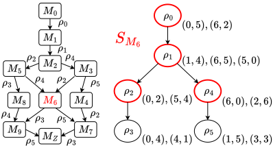
A stable matching always exists [Gale and Shapley, 1962] and the set of stable matchings M(I) forms a distributive lattice (see Fig. 1), where M0 is the manoptimal stable matching and MZ is the woman-optimal (man-pessimal) stable matching. M0 and MZ can be found in O(n2 ) time with Gale-Shapley algorithm, for example in Instance 1, M0 is defined by the pairs {(0, 5), (1, 4), (2, 6), (3, 3), (4, 1), (5, 0), (6, 2)}. The number of stable matchings is potentially exponential [Irving and Leather, 1986]; therefore it is not convenient to directly manipulate the set of stable matchings.
A rotation ρ is a sequence of pairs ((mk0 , wk0 ), ..., (mkl , wkl )), with l ∈N∗ and kl ∈{1, ..., n}, that represents the changes to operate in a stable matching to obtain another stable matching. In a rotation, the pairs (mki ,wki ) are eliminated and the pairs (mki ,wki+1 ) (modulo l) are produced (or generated). We denote M\ρ the operation of eliminating a rotation ρ from a stable matching M (which means we apply the changes represented by ρ). There is a partial order ◁ on the set of rotations R(I); indeed some rotations have to be eliminated before some others to get a stable matching. We call rotation digraph D(I) = (V,A) the Hasse diagram representing the partially ordered set (R(I),◁). We denote N -(ρ) = {ρ′ ∈ R(I) : ρ′ ◁ ρ} the predecessors of ρ, and N +(ρ) = {ρ′ ∈ R(I) : ρ ◁ ρ′ } the successors of ρ. We denote I(ρ) the set of rotations incomparable with ρ.
A fundamental result ([Gusfield and Irving, 1989]) is that there is a one-one correspondence between the stable matchings of M(I) and the closed subsets of (R(I),◁). Indeed, each stable matching M is characterised by a closed subset of rotations SM, and iteratively eliminating the rotations of SM (by respecting the partial order) fromM0 allow getting M, as illustrated by Fig. 1. For instance, M0 is represented by the empty set, and MZ by R(I).
Another important result is that each pair is generated in at most one rotation, and eliminated in at most one rotation.
One consequence is that the number of rotations is bounded by n(n - 1)/2, where n is the size of an SM instance. Also, the pairs that exist in at least one stable matching are called stable pairs, and the pairs that exist in all stable matchings are called fixed pair. In RSM we study the case where a pair becomes forbidden. Therefore, we denote P(I) the set of non-fixed stable pairs, which are the pairs that can be suppressed from a stable matching, that is there exists either a rotation producing it (denoted ρp) or a rotation eliminating it (denoted ρe). Then to suppress a non-fixed stable pair (m, w) we can either exclude ρp(m,w) or include ρe(m,w) in its characterising closed subset of R(I). Note that for pairs in M0 there is no rotation that produces them, and for pairs in MZ there is no rotation that eliminates them.
Example 1. If we are on M6 (Figure 1) defined by the pairs {(0, 4), (1, 5), (2, 0), (3, 3), (4, 1), (5, 2), (6, 6)} and we want to supress the pair (1, 5), we can either include ρ5 which eliminates (1, 5) or exclude ρ1 which generates (1, 5). However, excluding ρ1 implies excluding ρ2 and ρ4 to maintain the closed subset property. This leads to change four additionnal pairs in M6 (the men {0, 1, 2, 5, 6} have a new partner), while including ρ5 only leads to change one additionnal pair (the men {1, 3} have a new partner).
3 The Robust Stable Matching Problem
3.1 Definitions and First Properties
In our study, we consider the following NP-HARD problem introduced by [Genc et al., 2017]:
Name: Robust Stable Matching (RSM)
Instance: An SM instance
Objective: Finding a (1,b)-supermatch with the smallest b.
The distance between two stable matchings corresponds to the number of pairs that differ between them:
Definition 2 (Distance). Let I be an SM instance. The distance D between two stable matchings M and M ′ is defined as follows: D(M,M ′ ) = |M\M ′ |. Thus D(M,M ′ ) = D(M ′ ,M) and D(M,M) = 0.
In practice, we will manipulate the closed subsets of R(I), so we need to adapt the definition of the distance. Also, one can notice that the number of pairs that change is equal to the number of men (or women) that have a new partner, because a stable matching is a one-to-one matching:
Definition 3 (Characterised distance). Let I an SM instance. Let SM and SM′ two closed subsets of R(I). The characterised distance d is defined as follows: d(SM, SM′) = | ⋃ρ∈SM∆SM′ H(ρ)|. Where H(ρ) is the set of men concerned by the rotation ρ, and SM∆SM′ is the symmetric difference between SM and SM′ .
Then, with M and M ′ two stable matchings, SM and SM′ their characterising closed subsets of R(I), we have D(M,M ′ ) = d(SM, SM′ ). With Definition 3 we can compute the characterised distance d in O(|V|) time. It also has a number of interesting properties that are easy to demonstrate:
Lemma 1. (Increasing property) Let A, B, C and D be four closed subsets of R(I). If A∆B ⊆ C∆D then d(A,B) ≤ d(C, D).
Lemma 2. Let SM, SM′ and S be three closed subsets of R(I). SM′ ⊆ SM ⇒ d(SM′ , SM′ ∪ S) ≥ d(SM, SM ∪ S).
Lemma 3. Let SM, SM′ and S be three closed subsets of R(I). SM ⊆ SM′ ⇒ d(SM′ , SM′ ∩ S) ≥ d(SM, SM ∩ S).
Now, we define some particular closed subsets required to express several important results.
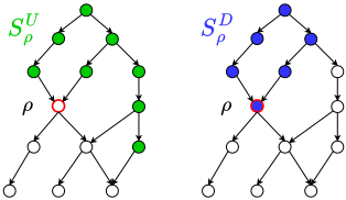
Definition 4 (UP and DOWN). For each ρ ∈ R(I), the closed subsets SU ρ and SD ρ are defined as follows:
- SU ρ is the maximal closed subset of rotations excluding ρ.
- SD ρ is the minimal closed subset of rotations including ρ. We denote Sup = {SU ρ : ρ ∈ R(I)} and Sdown = {SD ρ : ρ ∈ R(I)}
Remark. Let ρ ∈ R(I). SU ρ = R(I)\(N +(ρ) ∪ {ρ}) = N -(ρ) ∪ I(ρ) and SD ρ = N -(ρ) ∪ {ρ} (See Fig. 2). Therefore, Sup and Sdown can be computed in O(|V|3 ) time when knowing D(I).
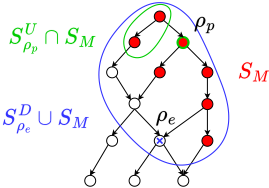
Theorem 1. Let M ∈ M(I) and SM be the closed subset characterising M. Let (m,w) ∈ M and ρp (resp. ρe) be the rotation that produces (m,w) (resp. eliminates). Note that one of these rotations may not exist. The nearest stable matching to M and not containing (m,w) is characterised by either SU ρp ∩ SM or SD ρe ∪ SM.
Proof. Let SM′ be a closed subset excluding ρp , then SM′ ⊆ SU ρp and so SM∆(SM ∩ SU ρp ) ⊆ SM∆SM′ . Hence d(SM , SM ∩ SU ρp ) ≤ d(SM , SM′ ) by Lemma 1.
Let SM′′ be a closed subset including ρe , then SD ρe ⊆ SM′′ and so SM∆(SM ∪ SD ρe ) ⊆ SM∆SM′′ . Hence d(SM, SM ∪ SD ρe ) ≤ d(SM , SM′′ ) by Lemma 1.
Figure 3: Illustration of Theorem 1
Finally, every stable matching that does not contain (m, w) is characterised by including ρe or excluding ρp.
Theorem 1 restates an important result from [Genc et al., 2017], but relies on our definition of the sets Sup and Sdown (Definition 4).
3.2 Mathematical Model
We call T (I) the set of transitional pairs, the pairs for which there is a rotation that eliminates them and a rotation that creates them. Therefore T (I) = P(I)\(M0 ∪MZ). Also, let M F 0 =M0 ∩P(I) be the pairs of M0 that can be forbidden, and M F Z = MZ∩P(I) the pairs of MZ that can be forbidden. Thus P(I) is the disjoint union of M F 0 , M F Z and T (I).
According to Theorem 1, the cost of suppressing a pair (m, w) from a stable matching M is defined as follows:
where SM is the closed subset of rotations characterising M. Remark. Let I be an SM instance and M a stable matching. ∀(m,w) ∈ P(I), (m,w) /∈M =⇒ bM(m,w) = 0.
Then, the robust score, or robust cost, of a stable matching M is defined as follows:
Finally, the RSM problem consists in finding a stable matchingM ∗ that minimises the robust cost:
And the optimal value is b∗ = b(M ∗ ).
3.3 Upper-Bound
Since we are studying a minimisation problem, we can evaluate the robust score of each stable matching to obtain an upper-bound on the optimal value. With Sup and Sdown we have access to many closed subsets for evaluation.
However, we only want to select a few number of stable matchings to get an upper-bound faster. To do so, we choose to evaluate M0, MZ and a median stable matching. Intuitively, a median stable matching is located in the "middle" of the partial order on M(I). So with M0 which is at the "beginning" and MZ at the "end", we roughly cover M(I). Here are two existing theorems about median stable matchings, slightly reformulated.
Theorem 2 ([Teo and Sethuraman, 1998]). Let T ⊆ M(I) and t = |T |. Let j ∈ {1, ..., t} and let αj,T denote the set of pairs obtained by assigning each man to his j th preferred woman in the multiset of all women he is matched to in the stable matchings of T . Then αj,T is a stable matching.
When t is odd, αt+1 2 ,T is called the unique median stable matching of T . When t is even, α t2 ,T (resp. α t2 +1,T ) is called the lower (resp. upper) median stable matching of T .
Theorem 3 ([Cheng, 2010]). Let T ⊆ M(I) and t = |T |. For each ρ ∈ R(I), let nρ,T = |{M ∈ T : ρ /∈ SM}|. Then ∀j ∈ {1, ..., t}, Rj,T (I) = {ρ ∈ R(I) : nρ,T < j} is a closed subset and characterises αj,T .
Theorem 3 allows to find a median stable matching for a subset of M(I) by analysing the rotations. Let Sup down be the multiset bringing together the closed subsets in Sup and Sdown (with possible repetitions). Let T up down denote the multiset of stable matchings characterised by the closed subsets of Sup down . We want to easily find the lower median stable matching of T up down , which we denote M up down .
Proof. Let ρ ∈ R(I). As a reminder, for each ρ′ ∈ R(I), SU ρ′ = N -(ρ′ ) ∪ I(ρ′ ) and SD ρ′ =N -(ρ′ ) ∪ {ρ′ }.
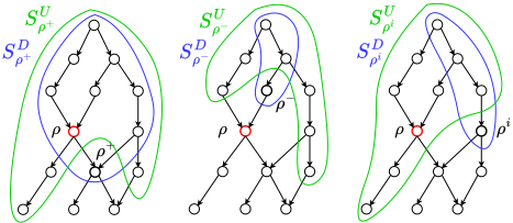
R(I) is the disjoint union of N +(ρ), N -(ρ), I(ρ) and {ρ}, so we analyse each case to count the number of closed subsets in Sup down that do not contain ρ (see Fig. 4).
- Let ρ+ ∈ N +(ρ), ρ ∈ SU ρ+ and ρ ∈ SD ρ+ .
- Let ρ- ∈ N -(ρ), ρ /∈ SU ρ- and ρ /∈ SD ρ- .
- Let ρi ∈ I(ρ), ρ ∈ SU ρi and ρ /∈ SD ρi .
- Also, ρ /∈ SU ρ and ρ ∈ SD ρ .
We deduce that nρ,T up down = 2 × |N -(ρ)| + |I(ρ)| + 1 = |SU ρ | + |SD ρ |. Finally, |T up down | = 2 × |R(I)|. So SM up down = R t2 ,T up down (with t = |T up down |), and by Theorem 3 it characterises α t2 ,T up down (which is M up down ).
Theorem 4 allows to find SM up down in O(|V|) time when Sup and Sdown are already known. Thus we can easily compute the robust score of M0, MZ and M up down , and provide an upper-bound b of the optimal value b∗ .
3.4 Computing the Robust Score Faster
Evaluating the robust score of a stable matching consists in finding the highest cost of the suppression of a pair, which implies calculating several distance values as we can see in the mathematical formulation (Section 3.2). Thus, computing the robust score can be done in O(n × |V|) time. However, we show that some pairs may always be more expensive to suppress than others. Therefore we might not need to calculate all the distances to get the robust cost. The theorems below explain in which case we can safely ignore some rotations or pairs. As a reminder, the only way to suppress a pair (m0,w0) ∈ M F 0 is by including the rotation ρ0 eliminating this pair. And the only way to suppress a pair (mZ,wZ) ∈ M F Z is by excluding the rotation ρZ producing this pair. Also, SM denotes the closed subset of rotations characterising the stable matching M.
Theorem 5. Let I be an SM instance.
∀(m0, w0) ∈ M F 0 , ∀M ∈M(I), ∀(m,w) ∈ P(I), ρe(m,w) ◁ ρ0 =⇒ bM(m,w) ≤ bM(m0,w0) where ρ0 is the rotation eliminating (m0, w0).
Proof. We assume that ρe(m, w) ◁ ρ0, then SD ρe(m,w) ⊆ SD ρ0 and so SM∆(SD ρe(m,w) ∪ SM) ⊆ SM∆(SD ρ0 ∪ SM). Hence d(SM , SD ρe(m,w) ∪ SM) ≤ d(SM, SD ρ0 ∪ SM) by Lemma 1, thus bM(m, w) ≤ bM(m0, w0).
Theorem 6. Let I be an SM instance.
∀(mZ, wZ) ∈ M F Z , ∀M ∈ M(I), ∀(m, w) ∈ P(I), ρZ ◁ ρp(m,w) =⇒ bM(m,w) ≤ bM(mZ,wZ)
where ρZ is the rotation producing (mZ, wZ).
Proof. We assume that ρZ ◁ ρp(m,w), then SU ρZ ⊆ SU ρp(m,w) and so SM∆(SU ρp(m,w) ∩SM) ⊆ SM∆(SU ρZ ∩SM ). Hence d(SM , SU ρp(m,w) ∩M) ≤ d(SM , SU ρZ ∩SM ) by Lemma 1, thus bM(m,w) ≤ bM(mZ,wZ).
Theorem 7. Let I be an SM instance. ∀(m, w) ∈ T (I), ∀M ∈ M(I), ∀(m′ , w′ ) ∈ T (I) such that ρp ◁ ρp(m′ , w′ ) and ρe(m′ , w′ ) ◁ ρe, we got bM(m′ , w′ ) ≤ bM(m, w) where ρp is the rotation producing (m, w), and ρe the rotation eliminating (m, w).
Proof. In the proofs of Theorems 5 and 6 we have shown that d(SM, SD ρe(m′ ,w′ ) ∪ SM) ≤ d(SM, SD ρe ∪ SM) and d(SM , SU ρp(m′ ,w′ ) ∩ SM) ≤ d(SM, SU ρp ∩ SM). Therefore bM(m′ , w′ ) ≤ bM(m, w).
Based on Theorems 5, 6 and 7, Algorithm 1 computes a reduced set Rup (resp. Rdown ) of rotations we need to exclude (resp. include), as well as a reduced set Pr of pairs we need to consider to compute the robust score of any stable matching.
Algorithm 1 starts by initialising the different variables in lines 1-4. Then, the loop at line 5 applies Theorem 5 to reduce Rdown , the one at line 8 applies Theorem 6 to reduce Rup , and the one at line 11 applies Theorem 7 to reduce Pr. The loop at line 16 checks if all up (resp. down) rotations generate (resp. eliminate) an irrelevant transitive pair, and if that is the case then it suppresses this rotation fromRup (resp. Rdown ).
Algorithm 1 Relevant pairs and rotations
Require: An instance I of SM, D(I), Sup and Sdown Ensure: Creating the sets Rup , Rdown and Pr 1: Rup ,Rdown ,Pr ←R(I),R(I),P(I) 2: for ρ ∈ R(I) do 3: Hup ρ ← |H(ρ)| 4: Hdown ρ ← |H(ρ)| 5: for (m,w) ∈M F 0 do 6: for ρ ∈ N -(ρe(m, w)) do 7: Rdown ← Rdown \{ρ} 8: for (m,w) ∈M F Z do 9: for ρ ∈ N +(ρp(m, w)) do 10: Rup ← Rup \{ρ} 11: for ((m,w), (m′ ,w′ )) ∈ T (I)2 do 12: if ρp(m,w) ◁ ρp(m′ ,w′ ) and ρe(m′ ,w′ ) ◁ ρe(m,w) then 13: Pr ← Pr\(m′ , w′ ) 14: Hup ρp(m′ ,w′ ) ← Hup ρp(m′ ,w′ ) - 1 15: Hdown ρe(m′ ,w′ ) ← Hdown ρe(m′ ,w′ ) - 1 16: for ρ ∈ R(I) do 17: if Hup ρ = 0 then 18: Rup ← Rup \{ρ} 19: if Hdown ρ = 0 then 20: Rdown ← Rdown \{ρ} 21: for (m,w) ∈ P(I) do 22: if ρp(m,w) /∈ Rup or ρe(m,w) /∈ Rdown then 23: Pr ← Pr\(m, w) return Rup , Rdown , PrFinally, the loop at line 21 checks Rup and Rdown to update Pr. Since T (I) has a size bounded by n2 , Algorithm 1 has a time complexity of O(n4 ) in the worst case.
3.5 Reducing the Size of the Search Space
The main difficulty of the stable marriage problems lies in the potentially exponential number of stable matchings [Irving and Leather, 1986], so that the search space can be very vast. By knowing an upper-bound b of the optimal value b∗ of the RSM problem, we show that it is possible to reduce the size of the search space. Indeed, in the theorems below we show that some rotations are present in every optimal solution, and some others in none of them.
Theorem 8. Let SM∗ be the closed subset of rotations characterising an optimal solution M ∗ , and let b be an upperbound of b∗ . Let ρ ∈ R(I) and ρ0 be the rotation eliminating a pair (m0, w0) ∈ M F 0 .
Proof. Let us prove the contraposition. We assume that ρ /∈ SM∗, then SM∗ ⊆ SU ρ . Firstly, by definition bM∗(m0,w0) = d(SM∗ , SM∗ ∪ SD ρ0 ), and then b∗ ≥ d(SM∗ , SM∗ ∪ SD ρ0 ) - 1. Secondly, according to Lemma 2, we have d(SM∗, SM∗ ∪ SD ρ0 ) ≥ d(SU ρ , SU ρ ∪ SD ρ0 ). Therefore, we deduce that
Algorithm 2 Lower and upper-bound of SM∗
Require: An instance I of SM, D(I), Sup and Sdown Ensure: Getting SLB and SUB 1: SLB, SUB ← ∅,R(I) 2: for (m,w) ∈M F 0 : ρe(m,w) ∈ Rdown do 3: for ρ ∈ SD ρe(m,w) do 4: if d(SU ρ , SU ρ ∪SD ρe(m,w) ) > b + 1 then 5: SLB ← SLB ∪ {ρ} 6: for (m,w) ∈M F Z : ρp(m,w) ∈ Rup do 7: for ρ ∈ R(I)\SU ρp(m,w) do 8: if d(SD ρ , SD ρ ∩SU ρp(m,w) ) > b + 1 then 9: SUB ← SUB\{ρ} return SLB, SUBTheorem 9. Let SM∗ be the closed subset of rotations characterising an optimal solution M ∗ , and let b be an upperbound of b∗ . Let ρ ∈ R(I) and ρZ be the rotation producing a pair (mZ,wZ) ∈ M F Z . Then, d(SD ρ , SD ρ ∩ SU ρZ ) > b +1 =⇒ ρ /∈ SM∗
Proof. Let us prove the contraposition. We assume that ρ ∈ SM ∗ , then SD ρ ⊆ SM∗. Firstly, by definition bM∗(mZ,wZ) = d(SM∗, SM∗ ∩ SU ρZ ), and then b∗ ≥ d(SM∗ , SM∗ ∩ SU ρZ ) - 1. Secondly, according to Lemma 3, we have d(SM∗ , SM∗ ∩ SU ρZ ) ≥ d(SD ρ , SD ρ ∩ SU ρZ ). Therefore we deduce that d(SD ρ , SD ρ ∩ SU ρZ ) ≤ b∗ + 1 and so d(SD ρ , SD ρ ∩SU ρZ ) ≤ b + 1
Based on Theorems 8 and 9, Algorithm 2 returns a lowerbound SLB and an upper-bound SUB on the closed subset SM ∗ characterising an optimal solution M ∗ .
Algorithm 2 starts by initialising SLB and SUB, then it consists of two main loops: one to increase SLB and the other to decrease SUB. The first one is based on Theorem 8 to add elements to SLB, and on Theorem 5 to compute only the relevant distances and quicken the algorithm. Similarly, the second main loop is based on Theorems 9 and 6 to rapidly suppress elements from SUB. Also, since the distance is computed in O(|V|) time, Algorithm 2 has a time complexity of O(n × |V|2 ) in the worst case.
Algorithms 1 and 2 have shown their efficiency as we explain in Section 6. But in the next Section, we prove that our results also hold for a larger family of instances.
4 Generalisation toMany-to-Many Instances
4.1 The Many-to-Many Problem (MM)
As for the SM problem, an instance of the Many-to-Many problem is a complete bipartite graph (U ∪ W,E) between men and women, with men having preferences over women and inversely. However, in the MM problem, both men and women can have several partners up to a maximum number called capacity. Each individual can have his own capacity. Similarly to the SM problem, the MM problem consists in finding a stable matching, which is a matching that has no blocking pair. Yet the definition of a blocking pair is slightly different:
Definition 5 (Blocking pair MM). Let I be an MM instance and M a matching. A pair (m,w) ∈ E\M is said to be a blocking pair for M iff the following conditions hold:
- m prefers w to his least preferred partner in M, or m has fewer partners in M than his capacity.
- w prefers m to her least preferred partner in M, or w has fewer partners in M than her capacity.
The MM problem generalises the SM problem but also the HR problem, where only one side can have several partners, and some works [Baıou and Balinski, 2000; Bansal et al., 2007; Eirinakis et al., 2012] have shown that a lot of results on SM also hold for MM. We reuse the same notations as for the SM problem that we recall now.
The set of stable matchings M(I) forms a lattice, with the existence of M0 and MZ. The partially ordered set of rotations (also called meta-rotations) (R(I),◁) exists too, and the stable matchings are characterised by the closed subsets of rotations. Each rotation generating a pair is a predecessor of the rotation eliminating it. Each pair has at most one rotation generating it and one rotation eliminating it. Each rotation generates as much pairs as it eliminates. Given two incomparable rotations, the sets of pairs they generate or eliminate are disjoint. These papers provide algorithms to get M0, MZ and the rotation digraph D(I) = (V,A) in O(n4 ) time that we will reuse in Section 6.
4.2 Robustness inMM
The distance between two stable matchings is the same as for SM (Definition 2), and we can extend it to the MM instances. However, we have to consider a generalised version of the characterised distance in SM (Definition 3):
Definition 6 (Generalised characterised distance). Let I be an MM instance. Let SM and SM′ two closed subsets of R(I). The generalised characterised distance dG is defined as follows: dG(SM, SM′) = ∣∣ ⋃ρ∈SM∆SM′ G(ρ) \ ⋃ρ∈SM∆SM′ E(ρ) ∣∣, where G(ρ) (resp. E(ρ)) is the set of pairs generated (resp. eliminated) by the meta-rotation ρ.
This distance is the number of newly generated and not eliminated pairs in the process of going from SM to SM′ (and inversely).
Lemma 4. (Increasing property) Let A, B, C and D be four closed subsets of R(I). If A∆B ⊆ C∆D then dG(A,B) ≤ dG(C, D).
Proof. As for SM instances, the more rotations we apply the more pairs we change. Due to the lack of space, the complete proof is detailed in the Technical Appendix.
All the theoretical results and algorithms obtained for the RSM problem on SM rely on the properties of the rotation digraph and the increasing property (Lemma 1). Since the MM instances also have a meta-rotation digraph with the same properties, and the generalised characterised distance dG verifies the increasing property too (Lemma 4), we can affirm that the theoretical results and algorithms obtained for the RSM problem on SM instances also hold for MM instances. Note that for the complexity of Algorithms 1 and 2 we have to replace n by n × c, where c is the highest capacity.
5 AConstraint ProgrammingModel
We present hereafter a CP model based on the set variables [Gervet, 1995; Gervet, 1997], and exploiting the algorithms 1 and 2 to solve the RSM problem extended to the MM instances. Before describing the model, we need to define the following two constraints. First, CLOSEDSUBSET(S,X) ensures that S is a closed subset of the partially ordered space X. Then, INDEXUNION(I, E, (Ri)i∈J) ensures that E = ⋃i∈I Ri with I ⊆ J. More details on these two constraints are given in the Technical Appendix.
The Model 1 is a formulation of the RSM problem. The set variable SM characterises the robust stable matching we are looking for. SM is bounded by SLB and SUB (2). (3) ensures that SM is a closed subset of R(I) represented by its Hasse diagram D(I). The variables with up as exponent, resp. down, are used to compute the cost of excluding, resp. including, a given rotation. The set variable ∆up ρ , resp. ∆down ρ , corresponds to the set of rotations that differs between SM and the nearest closed subset to SM excluding ρ (4), resp. including ρ (5). The set variable G up ρ , resp. G down ρ , represents the set of pairs generated by the rotations in ∆up ρ (6), resp. ∆down ρ (7). The set variable E up ρ , resp. E down ρ , represents the set of pairs eliminated by the rotations in ∆up ρ (8), resp. ∆down ρ (9). The integer variable Dup ρ , resp. Ddown ρ , counts the number of pairs in G up ρ \E up ρ (10), resp. G down ρ \E down ρ (11). The bM integer variables link a pair to the rotations that generate and eliminate it. The integer variable bM(τ) represents the cost of forbidding a pair τ = (m,w) in M (12). Finally, the objective is to minimise the highest cost (1). Without our preprocessing algorithms, Model 1 uses the initial values of SLB, SUB, Rup , Rdown and Pr (Algorithm 1, Line 1 and Algorithm 2, Line 1).
Note that our branching strategy consists in branching only on SM. Indeed, if SM is completely instantiated, all the other variables are fixed during propagation.
6 Experimental Results
In this section we conduct experiments on two models: a local search algorithm with random restarts LS from [Genc, 2019] (which is the state-of-the-art method for solving the RSM problem) implemented in Java (openjdk version 21.0.1) and generalised to the MM instances, and the CP model CP
Model 1 A model of the RSM problem.
| Minimise max{bM(m,w) : (m,w) ∈ Pr}- 1 | (1) | ||
| s.t.: SLB ⊆ SM ⊆ SUB | (2) | ||
| CLOSEDSUBSET(SM , D(I)) | (3) | ||
| ∆up ρ = SM\SU ρ , | ∀ρ ∈ Rup | (4) | |
| ∆down ρ = SD ρ \SM, | ∀ρ ∈ Rdown | (5) | |
| INDEXUNION(∆up ρ , Gup ρ , (G(ρ))ρ∈R(I)), | ∀ρ ∈ Rup | (6) | |
| INDEXUNION(∆down ρ , Gdown ρ , (G(ρ))ρ∈R(I)),∀ρ | ∈ Rdown | (7) | |
| INDEXUNION(∆up ρ , E up ρ , (E(ρ))ρ∈R(I)), | ∀ρ ∈ Rup | (8) | |
| INDEXUNION(∆down ρ , E down ρ , (E(ρ))ρ∈R(I)),∀ρ | ∈ Rdown | (9) | |
| Dup ρ = |Gup ρ \E up ρ |, | ∀ρ ∈ Rup | (10) | |
| Ddown ρ = |Gdown ρ \E down ρ |, | ∀ρ ∈ Rdown | (11) | |
| bM(τ ) = Ddown ρe(τ ) Dup ) | ∀τ ∈M F 0 ∩Pr ∀τ ∈M F Z ∩Pr | (12) | |
| ρp(τ min(Dup ρp(τ ) , Ddown ρe(τ) ) | ∀τ ∈ T (I) ∩Pr | ||
we provided in this paper and solved with Choco-solver [Prud'homme and Fages, 2022]. For both models, we consider two configurations: one where we only run PP1 (the preprocessing step allowing getting M0, MZ and D(I), that every rotation-based model has in common), and one where we run PP1 and our preprocessing step PP2 which consists of getting b and running Algorithms 1 and 2. We consider instances of SM (men and women have at most one partner), HR (only women can have several partners) and MM (both men and women can have several partners). For each instance size, we randomly generate 10 instances following a uniform distribution and report the mean statistics. This is the way instances of SM, HR and MM are usually generated in the literature [Genc, 2019; Manlove et al., 2007; Eirinakis et al., 2012]. We use an Intel(R) Xeon(R) Gold 6230 CPU with 2.10GHz and 3Go allocated RAM, and under Ubuntu 20.04.4 LTS.
For all instances, n is the number of men, m the number of women (equals to n when unspecified) and c the capacity (equals to 1 when unspecified). In the column PP, the value 1 indicates that PP1 is executed, the value 1+2 indicates that PP1 and PP2 are executed. The column time shows any cumulative preprocessing time. Then, the column space represents the size of the search space, it is equal to |R(I)| in the first configuration, and to |SUB| - |SLB| in the second one. bLS and timeLS (resp. bCP and timeCP ) indicate the best value found and the time required to obtain it with LS (resp. CP). proofCP indicates the time CP requires to prove the optimality once the best solution is found. When the optimal solution has been found for each of the 10 instances, the average value is labelled with "†". When the optimality of the solution has been proven on all 10 instances, "†" is replaced by "‡". All the time measures are in seconds.
In Tables 2-4, we observe the great improvements we have made on both models in all instances thanks to our preprocessing step. Indeed, when using the presolve algorithms, LS
| n | PP | time | space | b | bLS | bCP | timeLS | timeCP | proofCP |
|---|---|---|---|---|---|---|---|---|---|
| 500 | 1 | 0.85 | 92.8 | - | 346.2 | 345.8‡ | 112.04 | 4.10 | 1.29 |
| 1+2 | 0.95 | 5.7 | 354.8 | 346 | 345.8‡ | 0.15 | 0.039 | 0.039 | |
| 1000 | 1 | 6.42 | 150 | - | 756.8 | 755.8‡ | 191.07 | 33.27 | 10.47 |
| 1+2 | 6.75 | 12.1 | 778.3 | 755.8† | 755.8‡ | 0.94 | 0.29 | 0.02 | |
| 2000 | 1 | 51.99 | 267.3 | - | 1756.6 | 1637 | 226.65 | 380.62 | TimeOut |
| 1+2 | 53.40 | 11.1 | 1650 | 1633 | 1632.9‡ | 2.62 | 1.34 | 0.03 |
| n-m-c | PP | time | space | b | bLS | bCP | timeLS | timeCP | proofCP |
|---|---|---|---|---|---|---|---|---|---|
| 280- | 1 | 0.08 | 63.2 | - | 127.3 | 127.2‡ | 4.64 | 0.80 | 0.29 |
| 40-7 | 1+2 | 0.13 | 2.6 | 131.3 | 127.5 | 127.2‡ | 4.0E-4 | 0.006 | 0.005 |
| 500- | 1 | 0.22 | 130.2 | - | 289.1† | 289.1‡ | 76.95 | 5.97 | 2.451 |
| 63-8 | 1+2 | 0.33 | 6.3 | 297.1 | 289.1† | 289.1‡ | 0.062 | 0.037 | 0.005 |
| 840- | 1 | 0.32 | 195.2 | - | 478.8 | 477.4‡ | 84.41 | 27.50 | 8.47 |
| 70-12 | 1+2 | 0.45 | 5.2 | 485.6 | 477.7 | 477.4‡ | 1.5E-3 | 0.054 | 0.004 |
| n-c | PP | time | space | b | bLS | bCP | timeLS | timeCP | proofCP |
|---|---|---|---|---|---|---|---|---|---|
| 100- | 1 | 0.08 | 69.3 | - | 154.3† | 154.3‡ | 23.53 | 1.01 | 0.39 |
| 3 | 1+2 | 0.12 | 5.8 | 162.9 | 154.3† | 154.3‡ | 0.005 | 0.011 | 0.010 |
| 300- | 1 | 0.53 | 302.6 | - | 986.5 | 972.1‡ | 143.08 | 170.28 | 49.69 |
| 5 | 1+2 | 0.96 | 9 | 984.1 | 972.2 | 972.1‡ | 0.63 | 0.33 | 0.01 |
| 500- | 1 | 2.38 | 879.3 | - | 4183.7 | - | 109.46 | TimeOut | TimeOut |
| 10 | 1+2 | 5.43 | 14.2 | 3504.2 | 3476.9† | 3476.9‡ | 0.14 | 3.14 | 0.05 |
and CP are much faster (up to several thousand times faster on average to get the best solution) and give optimal or nearoptimal solutions. This is due to the great reduction of the search space, as we can see from the values of space, and to the acceleration of the evaluation speed (full results are in the Technical Appendix). The good quality of the upper-bound b (at most 5% away from the optimal value) is the reason why we can reduce this much the search space. Furthermore, our preprocessing time is very low and is largely compensated by the speed of the improved models. Finally, thanks to PP2 our CP model is able to find and prove optimal solutions even for large instances for which CP without PP2 timed out.
7 Conclusion
In this paper, we have established theoretical results on the Robust Stable Matching problem on SM instances. We have provided polynomial time algorithms for a preprocessing step that exploit these results. Also, we have generalised our theoretical results and algorithms to MM instances. We have shown experimentally that these algorithms allow to greatly improve the efficiency and the quality of any rotation-based model (via experiments on a heuristic and an exact method) solving the RSM problem on SM, HR and MM instances. The constraint programming model we provide, based on our presolve algorithms, is able to solve the problem exactly, even for large instances. In future work, it may be interesting to investigate the potential guarantees of these presolve algorithms, or possibly to find an approximate algorithm using a median stable matching. At last, this paper focuses on finding (1,b)-supermatches, so further studies could considerate the general case of finding (a,b)-supermatches, for which we do not know any polynomial-time method to evaluate the robust score, and the possibility to use similar presolve algorithms.
Acknowledgments
This publication has emanated from research conducted with the financial support of the Futur & Ruptures program co-granted by IMT, Institut Carnot TSN, Institut Carnot M.I.N.E.S. and Fondation Mines-T´el´ecom.
@inproceedings{ijcai2024p317,
  title     = {Polynomial Time Presolve Algorithms for Rotation-Based Models Solving the Robust Stable Matching Problem},
  author    = {Le Bozec-Chiffoleau, Sulian and Prud'homme, Charles and Simonin, Gilles},
  booktitle = {Proceedings of the Thirty-Third International Joint Conference on
               Artificial Intelligence, {IJCAI-24}},
  publisher = {International Joint Conferences on Artificial Intelligence Organization},
  editor    = {Kate Larson},
  pages     = {2860--2867},
  year      = {2024},
  month     = {8},
  note      = {Main Track},
  doi       = {10.24963/ijcai.2024/317},
  url       = {https://doi.org/10.24963/ijcai.2024/317},
}
TY - CPAPER TI - Polynomial Time Presolve Algorithms for Rotation-Based Models Solving the Robust Stable Matching Problem AU - Le Bozec-Chiffoleau, Sulian AU - Prud'homme, Charles AU - Simonin, Gilles T2 - Proceedings of the Thirty-Third International Joint Conference on Artificial Intelligence, IJCAI-24 PB - International Joint Conferences on Artificial Intelligence Organization PY - 2024 SP - 2860 EP - 2867 DO - 10.24963/ijcai.2024/317 UR - https://doi.org/10.24963/ijcai.2024/317 ER -Copied
Machine-readable versions of this paper, for tools and AI agents:





