
Effective Approach to LTLf Best-Effort Synthesis in Multi-Tier Environments
Proceedings of the Thirty-Third International Joint Conference on Artificial Intelligence. Main Track. Pages 3232-3240.
https://doi.org/10.24963/ijcai.2024/358
Keywords
- Knowledge Representation and Reasoning: KRR: Reasoning about actions
- Agent-based and Multi-agent Systems: MAS: Formal verification, validation and synthesis
Abstract
We consider an agent acting in a complex environment modeled through a multi-tiered specification, in which each tier adds nondeterminism in the environment response to the agent actions. In this setting, we devise an effective approach to best-effort synthesis, i.e., synthesizing agent strategies that win against a maximal set of possible environment responses in each tier. We do this in a setting where both the multi-tier environment and agent goal are specified in the linear temporal logic on finite traces (LTLf). While theoretical solution techniques based on automata on infinite trees have been developed previously, we completely side-step them here and focus on a DFA-based game-theoretic technique, which can be effectively implemented symbolically. Specifically, we present a provably correct algorithm that is based on solving separately DFA-based games for each tier and then combining the obtained solutions on-the-fly. This algorithm is linear, as opposed to being exponential, in the number of tiers and thus, it can graciously handle multi-tier environments formed of several tiers.
- [Alford et al., 2014] Ronald Alford, Ugur Kuter, Dana S. Nau, and Robert P. Goldman. Plan aggregation for strong cyclic planning in nondeterministic domains. Artificial In- telligence, 216:206-232, 2014.
- [Aminof et al., 2018] Benjamin Aminof, Giuseppe De Gia- como, Aniello Murano, and Sasha Rubin. Planning and synthesis under assumptions. arXiv, 2018.
- [Aminof et al., 2019] Benjamin Aminof, Giuseppe De Gia- como, Aniello Murano, and Sasha Rubin. Planning under LTL environment specifications. In ICAPS, pages 31-39, 2019.
- [Aminof et al., 2020] Benjamin Aminof, Giuseppe De Gia- como, Alessio Lomuscio, Aniello Murano, and Sasha Ru- bin. Synthesizing strategies under expected and excep- tional environment behaviors. In IJCAI, 2020. IJCAI
- [Aminof et al., 2021a] Benjamin Aminof, Giuseppe De Gia- como, Alessio Lomuscio, Aniello Murano, and Sasha Ru- bin. Synthesizing best-effort strategies under multiple en- vironment specifications. In KR, pages 42-51, 2021.
- [Aminof et al., 2021b] Benjamin Aminof, Giuseppe De Gia- como, and Sasha Rubin. Best-effort synthesis: Doing your best is not harder than giving up. In IJCAI, pages 1766- 1772, 2021. IJCAI
- [Aminof et al., 2023] Benjamin Aminof, Giuseppe De Gia- como, and Sasha Rubin. Reactive synthesis of dominant strategies. In AAAI, pages 6228-6235. AAAI Press, 2023.
- Krzysztof R. Apt and Erich Grädel, editors. Lectures in Game Theory for Computer Scientists. Cambridge University Press, 2011.
- [Bansal et al., 2020] Suguman Bansal, Yong Li, Lucas M. Tabajara, and Moshe Y. Vardi. Hybrid compositional rea- soning for reactive synthesis from finite-horizon specifica- tions. In AAAI, pages 9766-9774, 2020.
- [Bansal et al., 2022] Suguman Bansal, Giuseppe De Gia- como, Antonio Di Stasio, Yong Li, Moshe Y. Vardi, and Shufang Zhu. Compositional safety LTL synthesis. In VSTTE, volume 13800 of Lecture Notes in Computer Sci- ence, pages 1-19. Springer, 2022.
- [Bryant, 1992] Randal E. Bryant. Symbolic Boolean Ma- nipulation with Ordered Binary-Decision Diagrams. ACM Comput. Surv., 24(3):293-318, 1992.
- [Camacho et al., 2019] Alberto Camacho, Meghyn Bien- venu, and Sheila A McIlraith. Towards a unified view of AI planning and reactive synthesis. In ICAPS, pages 58- 67, 2019.
- [Cimatti et al., 2003] Alessandro Cimatti, Marco Pistore, Marco Roveri, and Paolo Traverso. Weak, strong, and strong cyclic planning via symbolic model checking. Arti- ficial Intelligence, 147:35-84, 2003.
- [Ciolek et al., 2020] Daniel Alfredo Ciolek, Nicolás D'Ippolito, Alberto Pozanco, and Sebastian Sardiña. Multi-tier automated planning for adaptive behavior. In ICAPS, pages 66-74. AAAI Press, 2020.
- [De Giacomo and Favorito, 2021] Giuseppe De Giacomo and Marco Favorito. Compositional approach to translate LTL f /LDL f into deterministic finite automata. In ICAPS, pages 122-130, 2021.
- [De Giacomo and Vardi, 2013] Giuseppe De Giacomo and Moshe Y. Vardi. Linear temporal logic and linear dynamic logic on finite traces. In IJCAI, pages 854-860, 2013. IJCAI
- [De Giacomo and Vardi, 2015] Giuseppe De Giacomo and Moshe Y. Vardi. Synthesis for LTL and LDL on finite traces. In IJCAI, pages 1558-1564, 2015. IJCAI
- [De Giacomo et al., 2020a] Giuseppe De Giacomo, Antonio Di Stasio, Francesco Fuggitti, and Sasha Rubin. Pure-past linear temporal and dynamic logic on finite traces. In IJ- CAI, pages 4959-4965. ijcai.org, 2020. IJCAI
- [De Giacomo et al., 2020b] Giuseppe De Giacomo, Antonio Di Stasio, Moshe Y Vardi, and Shufang Zhu. Two-stage technique for LTL f synthesis under LTL assumptions. In KR, volume 17, pages 304-314, 2020.
- [De Giacomo et al., 2023a] Giuseppe De Giacomo, Gian- marco Parretti, and Shufang Zhu. LTL f best-effort synthe- sis in nondeterministic planning domains. In ECAI, pages 533-540, 2023.
- [De Giacomo et al., 2023b] Giuseppe De Giacomo, Gian- marco Parretti, and Shufang Zhu. Symbolic LTL f best- effort synthesis. In EUMAS, pages 228-243, 2023.
- [Favorito and Zhu, 2023] Marco Favorito and Shufang Zhu. LydiaSyft: A compositional symbolic synthesizer for LTL f specifications. 2023.
- [Finkbeiner, 2016] Bernd Finkbeiner. Synthesis of reactive systems. Dependable Software Systems Eng., 45:72-98, 2016.
- [Fried et al., 2016] Dror Fried, Lucas M. Tabajara, and Moshe Y. Vardi. BDD-based Boolean functional synthesis. In CAV, pages 402-421, 2016.
- [Gabaldon, 2011] Alfredo Gabaldon. Non-Markovian con- trol in the situation calculus. Artificial Intelligence, 175:25-48, 2011.
- [Gale and Stewart, 1953] David Gale and Frank M Stewart. Infinite games with perfect information. Contributions to the Theory of Games, 2(245-266):2-16, 1953.
- [Geffner and Bonet, 2013] Hector Geffner and Blai Bonet. A Concise Introduction to Models and Methods for Auto- mated Planning. Morgan & Claypool, 2013.
- [Haslum et al., 2019] Patrik Haslum, Nir Lipovetzky, Daniele Magazzeni, and Christian Muise. An Introduction to the Planning Domain Definition Language. M&C, 2019.
- [Manna and Pnueli, 1990] Zohar Manna and Amir Pnueli. A hierarchy of temporal properties. In PODC, pages 377- 410, 1990.
- [Pnueli and Rosner, 1989] A. Pnueli and R. Rosner. On the synthesis of a reactive module. In POPL, page 179-190, 1989.
- [Pnueli, 1977] Amir Pnueli. The Temporal Logic of Pro- grams. In FOCS, pages 46-57, 1977.
- [Reiter, 2001] Raymond Reiter. Knowledge in Action: Logi- cal Foundations for Specifying and Implementing Dynam- ical Systems. MIT Press, 2001.
- [Somenzi, 2016] Fabio Somenzi. CUDD: CU Decision Di- agram Package 3.0.0. Universiy of Colorado at Boulder. 2016.
- [Zhu et al., 2017] Shufang Zhu, Lucas M. Tabajara, Jianwen Li, Geguang Pu, and Moshe Y. Vardi. Symbolic LTL f synthesis. In IJCAI, pages 1362-1369, 2017.
- [Zhu et al., 2020] Shufang Zhu, Giuseppe De Giacomo, Geguang Pu, and Moshe Y. Vardi. LTL f synthesis with fairness and stability assumptions. In AAAI, pages 3088- 3095, 2020.
References were extracted automatically from the PDF and may contain errors.
Full text extracted automatically from the PDF; figures, tables and equations may differ. The PDF is the version of record.
1 Introduction
There is a growing interest in Reasoning about Actions, Planning, and Sequential Decision Making on developing autonomous AI systems that can operate effectively in complex and dynamic environments where the level of nondeterminism is high. We typically assume that the AI system, i.e., the agent, has a single or flat model of the environment (specified, e.g., in the Situation Calculus [Reiter, 2001], or in PDDL [Haslum et al., 2019], or in Temporal Logics [Aminof et al., 2018; Camacho et al., 2019; Aminof et al., 2019]), which the agent uses to deliberate how to achieve its goals. However, accurately modeling such environments can be challenging, particularly when there is a high degree of uncertainty. Hence, the scientific community has been exploring the concept of multi-tier models of environment behavior, i.e., having simultaneously several models, or tiers, of the environment such that, in each tier the environment is more nondeterministic than in the previous one [Aminof et al., 2020; Ciolek et al., 2020; Aminof et al., 2021a]. For example, an agent may have a tier that represents the expected environment behavior, but also other tiers that represent increasingly nondeterministic deviations from that behavior, due to deteriorated or exceptional responses.
Given a multi-tier environment model, the agent simultaneously reasons on the effects of its actions in all tiers when deliberating what to do. This increases the robustness and adaptability of its operations when deployed in complex and uncertain environments. However, while the agent may have winning strategies (plans) to achieve its goals in the most deterministic tier, it may be impossible to have winning strategies also for the most nondeterministic tiers. This calls for notions of strategies that are less stringent than the usual ones used in Formal Methods [Finkbeiner, 2016], or in Planning [Geffner and Bonet, 2013].
One option is to introduce stochastic/quantitative aspects in the models and base reasoning on optimization with probabilistic guarantees [Geffner and Bonet, 2013]. But also in the non-quantitative setting there are interesting solutions, in particular that of best-effort strategies [Aminof et al., 2020; Aminof et al., 2021a; Aminof et al., 2021b]: if a strategy to win the goal against all possible environment responses does not exist, instead of giving up, we return a strategy that wins against a maximal set (though not all) of possible environment responses. Best-effort strategies are based on the game-theoretic rationality principle that a player (the agent) should not use a strategy that is "dominated" by another one (i.e., if another strategy fulfills the goal against more environment responses, then the player should adopt that strategy). Best-effort strategies have some notable properties: (i) they always exist, (ii) if a winning strategy exists, then besteffort strategies are exactly the winning strategies, (iii) for Linear Temporal Logic specifications both on infinite traces (LTL) [Pnueli, 1977] and on finite traces (LTLf ) [De Giacomo and Vardi, 2013], they can be computed in worst case 2EXPTIME, just as for winning strategies (best-effort synthesis is indeed 2EXPTIME-complete, just as is standard synthesis) [Aminof et al., 2021b].
These results extend to multi-tier environments. In particular, a strategy that is best-effort in all tiers of the multitier environment model always exists, i.e., there exists a strategy that in every tier wins against a maximal set of environment strategies. Moreover, such a strategy can be computed in 2EXPTIME for LTL/LTLf specifications. The latter result has been proved constructively in [Aminof et al., 2021a] by providing a solution technique based on automata on infinite trees. However that automata-based technique is not particularly promising for implementation.
Interestingly, in the case of flat environment models, one can resort to an alternative synthesis technique [Aminof et al., 2021b], which is a game-theoretic construction that can be implemented effectively, especially for LTLf . This technique is based on solving an adversarial and a cooperative game over an arena provided by the environment specification (and the agent goal) and then combining the two solutions.
In this paper, we focus on LTLf 1 . Using LTLf allows to specify every LTL guarantee specification for the goal and every LTL safety specification for the environment [Manna and Pnueli, 1990]. Notably, safety environment specifications are a generalization of nondeterministic planning domain specifications (for example, they allow for non-Markovian properties [Gabaldon, 2011]), e.g., written in PDDL making use of oneof (dropping preconditions in favor of conditional effects) [Haslum et al., 2019; Aminof et al., 2018; De Giacomo et al., 2023a].
Our first contribution is to show that the game-theoretic approach in [Aminof et al., 2021b] can be extended to handle multi-tier environments. Specifically, we show that we can combine adversarial and cooperative games for each tier of the environment and generate a strategy that is best-effort for all of them (Algorithm 1). However, by adopting such a basic technique, we obtain a game arena that is exponential in the number of tiers, limiting the applicability to only few tiers.
Our second contribution is to show that this exponential blowup in the number of tiers can be avoided. We present a refinement (Algorithm 2) of the basic technique, which is based on solving the games corresponding to an environment specification separately and combining the solutions on-thefly (in linear time) to obtain a strategy that step-wise returns the next action to be performed. The result is an algorithm that is linear in the number of environment specifications, and worst-case doubly exponential only in the size of the formulas specifying the goal and the environments (Theorem 6).
Our third contribution is to analyze two notable cases of multi-tier environments specified in LTLf : (i) the case in which all tiers share a (large) common base component, i.e., have the form Ei = Ec∧E ′ i , and (ii) the case in which, each tier is obtained by conjoining some further conditions to the previous one, i.e., Ei-1 = Ei ∧ E ′ i-1 . We exploit this additional structure, getting a construction that is even more scalable.
To show the practicality of the proposed approach, we provide symbolic implementations by leveraging the framework of [Zhu et al., 2017] and, using such implementations, perform an empirical evaluation on some scalable benchmarks.
2 LTLf Synthesis
A trace over an alphabet of symbols Σ is a finite or infinite sequence of elements from Σ. The empty trace is denoted
1 All techniques reported here also apply to LDLf [De Giacomo and Vardi, 2013] and pure-past LTL [De Giacomo et al., 2020a].
λ. Traces are indexed starting at zero, and we write π = π0π1 · · · . For a finite trace π, let lst(π) denote the index of the last element of π, i.e., lst(π) = |π| - 1.
Linear Temporal Logic on finite traces (LTLf ) is a specification language for expressing temporal properties on finite traces [De Giacomo and Vardi, 2013]. LTLf has the same syntax as LTL (which is instead interpreted over infinite traces [Pnueli, 1977]). Given a set AP of atomic propositions (aka atoms), the LTLf formulas over AP are generated by the following grammar: φ ::= a | φ ∧ φ | ¬φ | ◦φ | φU φ, where a ∈ AP. Here ◦ (Next) and U (Until) are temporal operators. We use standard Boolean abbreviations such as ∨ (or), ⊃ (implies), true and false. Moreover, we define the following abbreviations: ·φ ≡ ¬◦¬φ (Weak Next), ✸φ ≡ true U φ (Eventually), and ✷φ ≡ ¬✸¬φ (Always). The size of φ, written |φ|, is the number of its subformulas. Formulas are interpreted over finite traces π over the alphabet Σ = 2AP , i.e., the alphabet consisting of the propositional interpretations of the atoms. Thus, for 0 ≤ i ≤ lst(π), πi ∈ 2AP is the i-th interpretation of π. That an LTLf formula φ holds at instant i ≤ lst(π), written π, i |= φ, is defined inductively: 1. π, i |= a iff a ∈ πi (for a ∈ AP); 2. π, i |= ¬φ iff π, i ̸|= φ; 3. π, i |= φ1 ∧ φ2 iff π, i |= φ1 and π, i |= φ2; 4. π, i |= ◦φ iff i < lst(π) and π, i + 1 |= φ; and 5. π, i |= φ1 U φ2 iff ∃j such that i ≤ j ≤ lst(π) and π, j |= φ2, and ∀k, i ≤ k < j we have that π, k |= φ1. We say that π satisfies φ, written π |= φ, if π, 0 |= φ.
LTLf (reactive) synthesis [De Giacomo and Vardi, 2015] concerns finding a strategy to satisfy an LTLf goal specification. Goals are expressed as LTLf formulas over AP = Y ∪ X, where Y and X are disjoint sets of variables. Intuitively, Y (resp. X) is under the agent's (resp. environment's) control. Traces over Σ = 2Y∪X will be denoted π = (Y0 ∪ X0)(Y1 ∪ X1) . . . where Xi ⊆ X and Yi ⊆ Y for every i. Such infinite traces are called plays, and finite traces are called histories and represent a sequence of moves of the players ending in an environment move since we assume that the agent moves first.
An agent strategy is a function σag : (2X )∗ → 2Y mapping sequences of environment moves to an agent move. Similarly, an environment strategy is a function σenv : (2Y )+ → 2X mapping non-empty sequences of agent moves to an environment move. The domain of σag includes the empty sequence λ as we assumed that the agent moves first. A trace π is σag-consistent if Y0 = σag(λ) and Yj+1 = σag(X0 · · ·Xj) for every j ≥ 0. Analogously, π is σenv-consistent if Xj = σenv(Y0 · · · Yj) for every j ≥ 0. We define PLAY(σag, σenv) to be the unique (infinite) trace that is consistent with both σag and σenv.
Let φ be an LTLf formula over Y ∪ X. An agent strategy σag is winning for (aka enforces) φ if, for every environment strategy σenv, some finite prefix of PLAY(σag, σenv) satisfies φ. An agent strategy is cooperatively winning for φ if there exists an environment strategy σenv such that some finite prefix of PLAY(σag, σenv) satisfies φ. LTLf synthesis is the problem of finding an agent strategy σag that enforces φ, if one exists [De Giacomo and Vardi, 2015].
In this paper, we are interested in LTLf synthesis under environment specifications [Aminof et al., 2018]. Environment specifications describe some knowledge about how the environment works and are expressed as LTLf formulas E over Y ∪X . An environment strategy σenv is winning for (aka enforces) E if, for every agent strategy σag, every finite prefix of PLAY(σag, σenv) satisfies E. An environment specification is an LTLf formula E that is enforceable by some environment strategy. We denote by ΣE the set of environment strategies that enforce E.
Definition 1. [Aminof et al., 2018] Let φ (resp. E) be an LTLf formula over Y ∪X denoting an agent goal (resp. env spec). LTLf Synthesis under environment specifications is the problem of finding an agent strategy σag such that, for every environment strategy σenv ∈ ΣE, some finite prefix of PLAY (σag, σenv) satisfies φ, if one exists. Such a strategy is winning for φ in E (aka enforces φ in E)
An agent strategy σag is cooperatively winning for φ in E if there exists an environment strategy σenv ∈ ΣE such that PLAY (σag, σenv) has a finite prefix that satisfies φ.
Synthesis, both with LTLf environment specifications or not, is 2EXPTIME-complete [De Giacomo and Vardi, 2015; Aminof et al., 2018]. Synthesis under environment specifications is a generalization of synthesis which is obtained by taking E = true.
3 Best-Effort Strategies
We start by recalling basic notions on best-effort strategies [Aminof et al., 2020; Aminof et al., 2021b; Aminof et al., 2021a].
Definition 2. Let φ and E be LTLf formulas over Y ∪X denoting an agent goal and an environment specification, respectively, and let σ1 and σ2 be agent strategies. We say that σ1 dominates σ2, written σ1 ≥φ|E σ2, if, for every σenv ∈ ΣE, if some finite prefix of PLAY(σ2, σenv) satisfies φ then some finite prefix of PLAY(σ1, σenv) satisfies φ. Furthermore, σ1 strictly dominates σ2, written σ1 >φ|E σ2, if σ1 ≥φ|E σ2 and σ2 ̸≥φ|E σ1.
Intuitively, σ1 >φ|E σ2 means that σ1 does at least as well as σ2 against every environment strategy enforcing E and strictly better against at least one such strategy. An agent using σ2 is not doing its best, since it could achieve its goal against a strictly larger set of environment strategies using σ1. In this framework, a best-effort strategy is one which is not strictly dominated by any other strategy.
Definition 3. An agent strategy σ is best-effort, or maximal, for φ in E, written σ ∈ Maxφ|E , if there does not exist another agent strategy σ′ such that σ′ >φ|E σ.
Best-effort strategies also admit a local characterization that uses the notion of value of a history [Aminof et al., 2021b]. Intuitively, the value of a history h is: "winning", if the agent can enforce φ in E from h; otherwise, "pending", if the agent has a cooperatively winning strategy for φ in E from h; otherwise, "losing". With this notion, best-effort strategies are those that witness the maximum value of each history h consistent with them.
For a history h and an agent strategy σag, we denote by ΣE(h, σag) the set of environment strategies σenv enforcing E such that h is consistent with σag and σenv. For an agent strategy σag, we denote by HE(σag) the set of all histories h such that ΣE(h, σag) is non-empty, i.e., HE(σag) is the set of all histories that are consistent with σag and some environment strategy enforcing E. For h ∈ HE(σag) define:
- valφ|E(σag, h) = +1 ("winning"), if for every σenv ∈ ΣE (h, σag), PLAY(σag, σenv) has a finite prefix that satisfies φ; otherwise,
- valφ|E(σag, h) = 0 ("pending"), if for some σenv ∈ ΣE (h, σag), PLAY(σag, σenv) has a finite prefix that satisfies φ; otherwise,
- valφ|E(σag, h) = -1 ("losing").
Finally, we denote by valφ|E(h) the maximum of valφ|E(σag, h) over all σag such that h ∈ HE(σag) (we define valφ|E(h) only in case h ∈ HE(σ) for some σ). Here is the local characterization of best-effort strategies:
Theorem 1. [Aminof et al., 2021b] A strategy σag is besteffort for φ in E (i.e., σag ∈ Maxφ|E) iff valφ|E(σag, h) = valφ|E(h) for every h ∈ HE(σag).
4 Best-Effort Synthesis inMulti-Tier Environments
We now introduce best-effort synthesis in multi-tier environments, i.e., environment models consisting of several tiers, each allowing more nondeterminism than the previous one. Formally, an LTLf multi-tier environment specification (aka multi-tier environment model) is a tuple E = (E1, · · · , En) of LTLf environment tiers such that ΣEi ⊆ ΣEi+1 for every i (i ≤ i < n). In this framework, a best-effort strategy is one that is simultaneously best-effort for every tier.
Definition 4. Given an LTLf goal φ and an LTLf multitier environment specification E = (E1, · · · , En), best-effort synthesis is the problem of finding an agent strategy that is best-effort for φ in E, i.e. such that σag ∈ ⋂i Maxφ|Ei .
Unlike classic LTLf synthesis [De Giacomo and Vardi, 2015; Pnueli and Rosner, 1989], a best-effort strategy for an LTLf goal φ in a LTLf multi-tier environment specification E always exists, though computing it requires 2EXPTIME as in classic synthesis [Aminof et al., 2021a].
Theorem 2. [Aminof et al., 2021a] Let φ be an LTLf goal and E = (E1, · · · , En) an LTLf multi-tier environment specification. There exists σag ∈ ⋂i Maxφ|Ei , and it can be computed in 2EXPTIME in the size of φ, E1, · · · , En.
We now illustrate such notions in a simple Robot Navigation (in FOND domains) scenario [Cimatti et al., 2003; Alford et al., 2014] where an agent has to plan in spite of increasing nondeterminism.
Example 1. An autonomous agent is assigned the goal of delivering packages in a building by moving across rooms. Assume that there is a kid in the building who has keys to close some doors. It is easy to see that the agent goal may not be realizable as, e.g., the kid might lock the robot in a room. Hence, the agent could use a best-effort strategy. In this scenario, an LTLf environment describes the initial state, the transitions of the planning domain, and that the kid might close doors for which he has a key. Assume that the designer has no knowledge of which keys the kid holds. Then, the agent could be provided with several specifications describing the possible environment responses, each of which assumes that the kid holds some keys. In a multi-tier environment model, each tier assumes that the kid has more and more keys. A strategy σag that is best-effort in such a multi-tier environment will intuitively behave as follows: at every point in time, and for each environment specification, if the goal is enforceable (e.g., because the kid cannot prevent this) then σag will enforce it, and if the goal requires cooperation to achieve (e.g., because the kid has the keys to the relevant rooms) then σag will achieve the goal if the kid chooses to cooperate. The fact that such a strategy exists is non-trivial in general, and follows from Theorem 2.
5 Solving Best-Effort Synthesis inMulti-Tier Environments
While [Aminof et al., 2021a] provide a solution technique for best-effort synthesis in multi-tier domains, their technique is based on automata on infinite trees and is not well suited for efficient implementation. Here, we provide a different technique based on DFA games, as that for best-effort synthesis in a flat environment from [Aminof et al., 2021b], but extended to handle multi-tier environments.
Deterministic Finite Automata. For convenience, we separate the acceptance condition of automata from their structure. We define a deterministic transition system (aka transition system) as a tuple D = (Σ, S, s0, δ), where: Σ is a finite input alphabet (usually Σ = 2AP ); S is a finite set of states; s0 ∈ S is the initial state; and δ : S × Σ → S is the transition function. The size of D is the cardinality of S. Let α = α0α1 . . . αn be a finite trace over the alphabet Σ. The run of α in D is the finite sequence of states ρ = s0s1 . . . sn+1 such that s0 is the initial state of D and si+1 = δ(si, αi) for every i ≤ lst(α). We extend δ to be a function δ : S × Σ∗ → S as follows: δ(s, λ) = s, and if sn = δ(s, α0 . . . αn-1) then δ(s, α0 . . . αn) = δ(sn, αn).
Definition 5. The synchronous product of two transition systems Di = (Σ, Si, s(0,i), δi) (for i = 1, 2) over the same alphabet is the transition system PRODUCT(D1,D2) = D1 × D2 = (Σ, S, s0, δ) with: S = S1 × S2; s0 = (s(0,1), s(0,2)); and δ((s1, s2), x) = (δ(s1, x), δ(s2, x)). The product PRODUCT(D1, · · · ,Dn) = D1×· · ·×Dn is defined analogously for any finite sequence D1, · · · ,Dn of transition systems over the same alphabet.
A deterministic finite automaton (DFA) is a pair A = (D, F), where D = (Σ, S, s0, δ) is a deterministic transition system and F ⊆ S is the set of final states of the system. A trace α is accepted if δ(s0, α) ∈ F . The language of A is the set of traces that the automaton accepts.
Theorem 3. [De Giacomo and Vardi, 2013] Given an LTLf formula φ over AP, we can build a DFA, denoted TODFA(φ), whose size is at most 2EXP in |φ| and whose language is the set of finite traces that satisfy φ.
DFA Games. A DFA (D, F) in which Σ = 2Y∪X is called a DFA game. Here, D is called the game arena, and F is called the goal. The notions of plays, histories, and strategies from the Preliminaries Section apply also in this setting. A play is winning if it contains a finite prefix that is accepted by the DFA. Intuitively, winning a DFA game requires that F is visited at least once. An agent strategy σag is winning if, for every σenv, PLAY(σag, σenv) is winning. Furthermore, an agent strategy is cooperatively winning if there exists σenv such that PLAY(σag, σenv) is winning. Finally, an environment strategy σenv is winning if, for every σag, PLAY(σag, σenv) is not winning. The winning region (resp. cooperatively winning region) is the set of states s ∈ S for which the agent has a winning (resp. cooperatively winning) strategy in the game G ′ = (D′ , F), where D′ = (2Y∪X , S, s, δ), i.e., the same game as G, but with initial state s. The environment winning region is defined analogously. An agent strategy that is winning from every state in the agent winning region (resp. cooperatively winning region) is called uniform winning (resp. uniform cooperatively winning). Of special interest is the case where the agent strategy can be derived from a function κag : S → 2Y , called a positional strategy, mapping states of the game to agent moves. While a positional strategy is not formally an agent strategy (i.e., a function from sequences of environment moves to agent moves), it induces one as follows: STRATEGY(D, κag)(h) = κag(δ(s0, h)). The pair (D, κag) is sometimes called a transducer, i.e., a deterministic transition-system with output. Solving a DFA game is the problem of computing the agent winning (resp. cooperatively winning) region and determining a positional winning strategy (resp. positional cooperatively winning) strategy, written (W, κag) = SOLVEADV(D, F) (resp. (W ′ , γag) = SOLVECOOP(D, F)). Games played over DFAs are determined, meaning that the agent winning region and the environment winning region partition the state space [Gale and Stewart, 1953]. DFA games can be solved in linear time in the size of the game arena through a least-fixpoint computation [Apt and Gr¨adel, 2011]. The environment winning region is denoted ENVWIN(D, F).
Sometimes, transitions must be constrained to those that do not allow the game to leave a set of states:
Definition 6. Let D = (Σ, S, s0, δ) be a transition system and S′ ⊆ S a non-empty set of states. The restriction of D to S′ is the transition system RESTRICT(D, S′ ) = (Σ, S′ ∪ {sink}, s0, δ′ ) where, for every a ∈ Σ, δ′ (s, a) = sink if s = sink or δ(s, a) ̸∈ S′ , and δ′ (s, a) = δ(s, a) otherwise.
Solution Technique - Basic Version. As a first step towards developing our solution, we first review the core step in [Aminof et al., 2021b; De Giacomo et al., 2023b] 2 for the
2 We observe that in [Aminof et al., 2021b; Aminof et al., 2023] the environment moves first. This causes a mismatch between the automata constructed in the algorithms of those papers and the local characterization. While the local characterization talks about histories ending in environment moves, finite runs in automata correspond to histories ending in agent moves. This mismatch causes a bug in the algorithms of those papers. This bug can be fixed by having the agent move first, as we do in this paper. If one wishes for the
Algorithm 0 SYNTHPOS(φ, E)
Input: LTLf goal φ and an env. specification E Output: goal DFAAφ; env. DFAAE; winning regionW; cooperatively winning region W ′ ; positional winning strategy κ; positional cooperatively winning strategy γ
- 1: Aφ = TODFA(φ); AE = TODFA(E) Say Aφ = (Dφ, Fφ) and AE = (DE , FE )
- 2: D = PRODUCT(DE,Dφ)
- 3: Let:
- FE⊃φ = {(sE, sφ) | sE ∈ FE ⊃ sφ ∈ Fφ}
- F¬E = {(sE, sφ) | sE ̸∈ FE}
- FE∧φ = {(sE, sφ) | sE ∈ FE ∧ sφ ∈ Fφ}
- 4: (W, κ) = SOLVEADV(D, FE⊃φ)
- 5: V = ENVWIN(D, F¬E)
- 6: D′ = RESTRICT(D, V )
- 7: (W ′ , γ) = SOLVECOOP(D′ , FE∧φ)
- 8: Return (Aφ,AE,W,W ′ , κ, γ)
single environment LTLf best-effort synthesis problem, encapsulated in Algorithm 0. That allows one to compute a positional strategy as follows: it maps a state s in D = DE ×Dφ to κ(s) if s ∈ W, to γ(s) if s ∈ W ′ \W, and is arbitrary otherwise. Intuitively, the histories whose induced runs in D that pass or end in a state in W have value +1 (as witnessed by κ), those ending in a state in W ′ \ W have value 0 (as witnessed by γ), and the rest have value -1. The correctness is a consequence of the local characterization (Theorem 1).
With the auxiliary procedure Algorithm 0 in place, we are ready to present our solution technique. For we make no effort to gain maximal efficiency, which we will do in the next section, this solution should be thought of as a conceptual solution and not yet a blueprint for implementation. The technique is detailed in Algorithm 1 and returns a strategy obtained by combining the solutions of simple (adversarial and cooperative) DFA games, two for each environment specification Ei, computed in Step 1 by calling Algorithm 0. These strategies are combined into a positional strategy over the Cartesian product of all games computed in Step 3. Algorithm 1 exploits the fact the environment is given in the form of a multi-tier environment, i.e., ΣE1 ⊆ · · · ⊆ ΣEn , as follows. Suppose k < i. Then, an agent strategy that wins for φ in Ei also wins for φ in Ek since winning against all the strategies in ΣEi also wins against all the strategies in the subset ΣEk . Similarly, an agent strategy that cooperatively wins for φ in Ek also cooperatively wins for φ in Ei since a cooperating environment strategy in ΣEk is also in ΣEi . Intuitively, histories whose induced runs in the product D that pass or end in a state whose j-th coordinate is in Wj (where j is computed in Step 3) have value +1 for each of the environment specifications E1 up to Ej, and have value 0 for each of the environment specifications Ej+1 up to En; of the remaining histories, those ending in a state whose ℓ-th coordinate is
environment to move first, we can easily change the specification so that it ignores the first agent move. Alternatively, we can modify the automata construction by adding intermediate states in each transition that correspond to half time-steps after the environment move but before the corresponding agent move.
Algorithm 1 MULTIENVBESYNTH(φ, E1, · · · , En)
Input: LTLf goal φ and a multi-tier env. E = (E1 · · · En)
Output: Agent strategy σ that is best-effort for φ in E
- 1: For i = 1 . . . n: (Aφ, AEi , Wi, W ′ i , κi, γi) = SYNTHPOS(φ, Ei)3 Say Aφ = (Dφ, Fφ), Dφ = (2Y∪X , Sφ, sφ, δφ) Say AEi = (DEi , FEi ), DEi = (2Y∪X , SEi , sEi , δEi ) 2: D = PRODUCT(DE1 , · · · ,DEn ,Dφ)
- Say S = SE1 × · · · × SEn × Sφ
- 3: Define a positional strategy ν on S as follows. For s = (s1, · · · , sn, t) ∈ S:
- j = max{i : (si, t) ∈Wi}
- ℓ = min{i : (si, t) ∈W ′ i }
- if j exists then define ν(s) = κj(sj, t)4 else if ℓ exists then define ν(s) = γℓ(sℓ, t) else define ν(s) = Y (i.e., arbitrarily) endif
- 4: Return STRATEGY(D, ν)
in W ′ ℓ have value 0 for each of the environment specifications Eℓ up to En, and otherwise have value -1. The following theorem shows the correctness of the solution technique above:
Theorem 4. Algorithm 1 returns a strategy in ∩i≤nMaxφ|Ei .
6 Advanced Solution Technique
Although Algorithm 1 is correct, its runtime grows exponentially in n, the number of tiers in the multi-tier environment. Indeed, Algorithm 1 returns an agent strategy represented as a transducer with state space SE1 ×· · ·×SEn ×Sφ, where Sφ is the state space of Aφ and, for every i, SEi is the state space of AEi . The size of this state space grows exponentially in n. Constructing the positional strategy ν requires searching the whole state space (Step 3), and hence exponential time in n. Such exponential dependency limits the applicability of Algorithm 1 to best-effort synthesis problems with just few tiers. However, the ideas at the base of Algorithm 1 can be refined to avoid the exponential blow-up.
To do so, we substitute Algorithm 1 with Algorithm 2. The key difference is that we avoid the construction of the Cartesian product and instead return a strategy that determines onthe-fly, at each instant, the next action to perform by scanning in linear time the regions Wi and W ′ i (for 1 ≤ i ≤ n) and choosing a suitable output from the strategies κi and γi. With this technique, the cost of computing the output best-effort strategy is just linear in n (while remaining double exponential in the size of the LTLf formulas E1, · · · , En, φ), as well as the time cost for executing, at any instant, the output strategy. Since it is easy to see that the strategy returned by Algorithm 2 is equivalent to the strategy returned by Algorithm 1, from Theorem 4 we get the correctness of Algorithm 2.
Theorem 5. Algorithm 2 returns a strategy in ∩i≤nMaxφ|Ei .
Complexity. By analyzing Algorithm 2 we see that, while its complexity is 2EXPTIME in the LTLf formulas (as classic synthesis), it depends linearly on the number of tiers:
2 In fact, we only need to call TODFA(φ) once.
4 Recall that by Alg 0, the domains of κi and γi are SEi ×Sφ.
Algorithm 2 ONTHEFLYBESYNTH(φ, E1, · · · , En)
- Input: LTLf goal φ and a multi-tier env. E = (E1 · · · En) Output: Agent strategy σ that is best-effort for φ in E 1: For i = 1 . . . n: (Aφ, AEi , Wi, W ′ i , κi, γi) = SYNTHPOS(φ, Ei)2 Say Aφ = (Dφ, Fφ), Dφ = (2Y∪X , Sφ, sφ, δφ) Say AEi = (DEi , FEi ), DEi = (2X∪Y , SEi , sEi , δEi ) 2: Return the following best-effort strategy: While true: 1. j = max{i : (sEi , sφ) ∈Wi} 2. ℓ = min{i : (sEi , sφ) ∈W ′ i } 3. if j exists, output Y = κj(sEj , sφ) else if ℓ exists, output Y = γℓ(sEℓ , sφ) else output Y = Y endif 4. On environment's choice X ⊆ X : · Update sφ = δφ(sφ, Y ∪X) · For i = 1 . . . n: update sEi = δEi (sEi , Y ∪X)
Theorem 6. Let φ be an LTLf goal and E = (E1, · · · , En) a multi-tier environment specification. Then Algorithm 2 computes a strategy σ ∈ ⋂i Maxφ|Ei in 2EPXTIME in the size of φ, E1, · · · , En and in linear time in n, the number of tiers in the multi-tier environment.
Specifically, Algorithm 2 finds, at each instant (history), the next agent move (assignment of the Y) in linear time in the number of tiers, i.e., Algorithm 2 (differently form Algorithm 1) scales graciously as the number of tiers grows.
Interestingly, the computations in Step 1 of Algorithms 1 and 2 can be done in parallel. The n + 1 steps for computing the DFAs of the goal and the n environment specifications can be done in parallel; the n steps for computing the regions Wi and the strategies κi can be done in parallel; the n steps for computing the regions W ′ i and the strategies γi can be done in parallel. As a result, if n+1 processors are available, handling multi-tier environments is virtually for free, i.e., costs the same as handling the most computationally expensive tier.
These features suggest that Algorithm 2 is suited for efficient implementation, as confirmed empirically in Section 8.
7 Notable Cases
Before turning to implementation and experimental evaluation, we consider two notable cases of multi-tier environment models, for which we can offer further optimizations.
Multi-Tier Environments with a Common Base. In this case we have a (large) common base Ec that is common to all tiers. That is, each tier Ei is specified as conjunction of Ec with some additional LTLf specification E ′ i . Formally, multitier environments with a common base have the form: for every i s.t. 1 ≤ i ≤ n, Ei = Ec∧E ′ i , where ΣE ′1 ⊆ · · · ⊆ ΣE ′n .
Multi-Tier Environments with Conjunctive Refinements. Next, we consider multi-tier environments consisting of tiers that conjoin further constraints to the previous tier, becoming more determined. That is, the base environment is En, and each tier Ei refines Ei+1 with some conjunct E ′ i . Formally, multi-tier environments with conjunctive refinements have the form: for every i s.t. 1 ≤ i < n, Ei = Ei+1 ∧ E ′ i .
Exploiting Structure in Notable Cases. By taking advantage of the syntactic structure of these notable cases, we can devise optimized variants of Algorithm 2 that construct more efficiently the DFAs of the tiers. To do this, we exploit the following composition technique, whose correctness follows immediately by the notion of product of transition systems:
Theorem7. Given n LTLf formulas ψi, let ψ = ∧1≤i≤n ψi. If Aψi = (Dψi , Fψi ) is a DFA recognizing ψi (for 1 ≤ i ≤ n), then the DFA Aψ = (Dψ, Fψ) recognizes ψ: Dψ = PRODUCT(Dψ1 , · · · ,Dψn ) and Fψ = Fψ1 × · · · ×Fψn
With Theorem 7, we can construct the DFAs of the tiers as follows: (i) we construct the DFA of the base conjunct, i.e., Ec and En, respectively; (ii) we construct the DFAs of the conjuncts E ′ i ; (iii) we compose the obtained DFAs to construct the DFAs of the environment tiers. Constructing and composing the DFAs of the various conjuncts takes less time than transforming every tier into a DFA as a whole, especially if the size of the least refined tier is large and dominates that of the other conjuncts. This is confirmed empirically in Section 8.
8 Implementation and Evaluation
We implemented Algorithm 2 in a tool called MtSyft 5 , leveraging the symbolic LTLf synthesis framework [Zhu et al., 2017], at the base of state-of-the-art LTLf synthesis tools [Bansal et al., 2020; Favorito and Zhu, 2023]. We also developed variants of MtSyft customized for the two notable cases above, called cb-MtSyft and conj-MtSyft. In MtSyft, we build the minimized explicit-state DFAs of LTLf formulas with LYDIA [De Giacomo and Favorito, 2021], which is among the best performing tools publicly available for LTLf -to-DFA conversion. We code Boolean functions representing transitions and final states of symbolic DFAs by BDDs [Bryant, 1992] with the BDD library CUDD 3.0.0 [Somenzi, 2016]. We compute the positional strategies for the DFA-games through Boolean synthesis [Fried et al., 2016].
Setup. Experiments were run on a laptop with an operating system 64-bit Ubuntu 20.04, 3.6 GHz CPU, and 12 GB of memory. Timeout was set to 300 seconds.
Benchmark. To evaluate the performance of our implementations, we devised an extension of the counter game benchmarks presented in [De Giacomo et al., 2020b; Zhu et al., 2020] to construct multi-tier environment specifications. The counter game involves a k-bit counter as follows: (i) at each round, the environment chooses whether to request an increment of the counter (add), and the agent chooses whether to grant such a request or not; (ii), the counter is initialized with all bits set to 0, and the agent goal is for the counter to have all bits set to 1; (iii) multi-tier environment specifications define possible policies according to which the environment issues increment requests. Specifically, environment specifications are LTLf formulas E1 = add, and for m ≥ 2, Em = Em-1 ∧ ·· · · · ·add, where there are m - 1 occurrences of · in Em. In our experiments, the environment issues between 1 and 100 increment requests (1 ≤ m ≤ 100). Given a k-bits counter and an environment specification Em, the realizability of the agent goal (existence of a winning strategy for the goal) depends on k and m: if m ≥ 2k -1, the goal is realizable. Regardless of the realizability of the agent goal, a best-effort (possibly winning) strategy for the agent is to accept all environment increment requests.
5 https://github.com/GianmarcoDIAG/MtSyft
| Bits | Coverage | Avg. | RT (secs) | |
|---|---|---|---|---|
| MtSyft | cb-MtSyft | MtSyft | cb-MtSyft | |
| 1 | 82 | 82 | 50.98 | 54.92 |
| 2 | 82 | 82 | 55.85 | 51.46 |
| 3 | 81 | 83 | 52.04 | 54.95 |
| 4 | 80 | 82 | 49.55 | 53.40 |
| 5 | 82 | 84 | 55.75 | 57.99 |
| 6 | 82 | 82 | 58.84 | 55.53 |
| 7 | 81 | 80 | 64.05 | 57.64 |
| 8 | 76 | 77 | 73.42 | 74.94 |
| 9 | 0 | 0 | - | - |
| 10 | 0 | 0 | - | - |
| Total | 646 | 652 | ||
Our benchmark consists of counter games with at most 10bits. For each game, we constructed multi-tier environments with n tiers as follows: (i) we fixed a base conjunct Eℓ; (ii) stacked the tiers Eℓ, · · · , Eℓ+n-1 in increments of 1. As base conjucts, we considered E1, and E10 to E90 in increments of 10. In total, our benchmark consists of about 5600 instances.
Empirical Results. We performed experiments to assess: (i) the practical feasibility of best-effort synthesis in multitier environments as the number of tiers grows; and (ii) further scalability improvement obtainable exploiting the special structure of the two notable cases.
Table 1 shows the performance of MtSyft in counter game instances with number of tiers between 1 and 100 (1 ≤ n ≤ 100) where E1 is the base conjuct. We can see that MtSyft, run on a laptop, solves at most 8-bits counter games up to 76 tiers within the 300 secs timeout. For 8-bits counter games (or lower) the computational bottleneck is converting LTLf tier specifications into DFAs. Instead, solving the single games and composing the synthesized positional strategies into a the best-effort strategy (expressed as the while-program returned by Algorithm 2) brings only a minor computational overhead. For 9-bits and 10-bits counter games, MtSyft reaches the timeout while converting the LTLf goal itself (i.e., the counter specification) into a DFA (as opposed to the tiers). This is an excellent scalability result with respect to the number of tiers and confirms the practical feasibility of the synthesis in multi-tier environments. Table 1 includes the performance of cb-MtSyft as well, but the size of the base conjunct is too small to observe a significant scalability improvement.
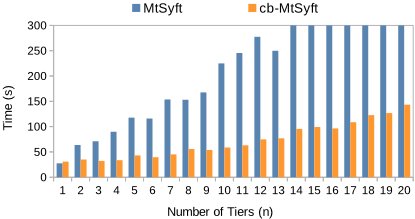
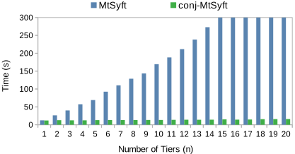
Figure 1 shows the performance comparison of MtSyft and cb-MtSyft in 8-bits counter games with base conjunct E80 (i.e., it has 80 successive increment request) and number of tiers between 1 and 20 (hence, going from E80 to E100). The results show that cb-MtSyft successfully solves all the considered instances, while MtSyft reaches the timeout when n = 14. In the solved instances, cb-MtSyft scales much better than MtSyft by exploiting the structure of the multitier environment to more efficiently construct the DFAs of the tiers. Figure 2 shows an analogous result on the performance comparison of MtSyft and conj-MtSyft in 1-bit counter games with base conjunct E80 and number of tiers between 1 and 20. We get the same performance up to 3-bits counters, then for 4-bits on it goes in time out. The reason is that our implementation does the conjunctions symbolically without minimizing the result, i.e., the product DFA grows exponentially in the number of conjuncts. To avoid the exponential blowup, one should adopt a more sophisticated way of handling conjunctions, as in [Bansal et al., 2020; Bansal et al., 2022].
9 Conclusion
We developed an effective technique to solve LTLf best-effort synthesis in multi-tier environments which allow for increasing nondeterminism. In our framework, we have considered a single goal for all tiers. However, it is also of interest to consider the case in which, as tiers become more undetermined, also the goal is weakened. For instance, the agent may have a primary goal that requires a certain type of environment behavior, but also secondary goals that can be achieved even if the environment does not behave as expected. This was studied for PDDL planning in [Ciolek et al., 2020]. We believe that the general approach presented here can be extended to handle this case as well. We leave the details for future work.
Acknowledgments
This work is supported in part by the ERC Advanced Grant WhiteMech (No. 834228), the EU ICT-48 2020 project TAILOR (No. 952215), the PRIN project RIPER (No. 20203FFYLK), and the PNRR MUR project FAIR (No. PE0000013). Gianmarco Parretti is supported by the Italian National Ph.D. on Artificial Intelligence at Sapienza.
@inproceedings{ijcai2024p358,
  title     = {Effective Approach to LTLf Best-Effort Synthesis in Multi-Tier Environments},
  author    = {Aminof, Benjamin and De Giacomo, Giuseppe and Parretti, Gianmarco and Rubin, Sasha},
  booktitle = {Proceedings of the Thirty-Third International Joint Conference on
               Artificial Intelligence, {IJCAI-24}},
  publisher = {International Joint Conferences on Artificial Intelligence Organization},
  editor    = {Kate Larson},
  pages     = {3232--3240},
  year      = {2024},
  month     = {8},
  note      = {Main Track},
  doi       = {10.24963/ijcai.2024/358},
  url       = {https://doi.org/10.24963/ijcai.2024/358},
}
TY - CPAPER TI - Effective Approach to LTLf Best-Effort Synthesis in Multi-Tier Environments AU - Aminof, Benjamin AU - De Giacomo, Giuseppe AU - Parretti, Gianmarco AU - Rubin, Sasha T2 - Proceedings of the Thirty-Third International Joint Conference on Artificial Intelligence, IJCAI-24 PB - International Joint Conferences on Artificial Intelligence Organization PY - 2024 SP - 3232 EP - 3240 DO - 10.24963/ijcai.2024/358 UR - https://doi.org/10.24963/ijcai.2024/358 ER -Copied
Machine-readable versions of this paper, for tools and AI agents:





