
ParsNets: A Parsimonious Composition of Orthogonal and Low-Rank Linear Networks for Zero-Shot Learning
Proceedings of the Thirty-Third International Joint Conference on Artificial Intelligence. Main Track. Pages 4062-4070.
https://doi.org/10.24963/ijcai.2024/449
Keywords
- Machine Learning: ML: Cost-sensitive learning
- Machine Learning: ML: Ensemble methods
- Machine Learning: ML: Learning sparse models
- Machine Learning: ML: Few-shot learning
Abstract
This paper provides a novel parsimonious yet efficient design for zero-shot learning (ZSL), dubbed ParsNets, in which we are interested in learning a composition of on-device friendly linear networks, each with orthogonality and low-rankness properties, to achieve equivalent or better performance against deep models. Concretely, we first refactor the core module of ZSL, i.e., the visual-semantics mapping function, into several base linear networks that correspond to diverse components of the semantic space, wherein the complex nonlinearity can be collapsed into simple local linearities. Then, to facilitate the generalization of local linearities, we construct a maximal margin geometry on the learned features by enforcing low-rank constraints on intra-class samples and high-rank constraints on inter-class samples, resulting in orthogonal subspaces for different classes. To enhance the model's adaptability and counterbalance the over-/under-fittings, a set of sample-wise indicators is employed to select a sparse subset from these base linear networks to form a composite semantic predictor for each sample. Notably, maximal margin geometry can guarantee the diversity of features and, meanwhile, local linearities guarantee efficiency. Thus, our ParsNets can generalize better to unseen classes and can be deployed flexibly on resource-constrained devices.
- [Akata et al., 2015] Zeynep Akata, Scott Reed, Daniel Wal- ter, Honglak Lee, and Bernt Schiele. Evaluation of out- put embeddings for fine-grained image classification. In IEEE/CVF Conference on Computer Vision and Pattern Recognition, pages 2927-2936, 2015.
- [Chen et al., 2021a] Shiming Chen, Guosen Xie, Yang Liu, Qinmu Peng, Baigui Sun, Hao Li, Xinge You, and Ling Shao. Hsva: Hierarchical semantic-visual adaptation for zero-shot learning. In Advances in Neural Information Processing Systems, pages 16622-16634, 2021.
- [Chen et al., 2021b] Zhi Chen, Yadan Luo, Ruihong Qiu, Sen Wang, Zi Huang, Jingjing Li, and Zheng Zhang. Se- mantics disentangling for generalized zero-shot learning. In IEEE/CVF International Conference on Computer Vi- sion, pages 8712-8720, 2021.
- [Chen et al., 2023] Dubing Chen, Yuming Shen, Haofeng Zhang, and Philip HS Torr. Deconstructed generation- based zero-shot model. In Proceedings of the AAAI Con- ference on Artificial Intelligence, volume 37, pages 295- 303, 2023.
- [Farhadi et al., 2009] Ali Farhadi, Ian Endres, Derek Hoiem, and David Forsyth. Describing objects by their attributes. In Computer Vision and Pattern Recognition, 2009. CVPR 2009. IEEE Conference on, pages 1778-1785. IEEE, 2009.
- [Feng et al., 2022] Yaogong Feng, Xiaowen Huang, Pengbo Yang, Jian Yu, and Jitao Sang. Non-generative generalized zero-shot learning via task-correlated disentanglement and controllable samples synthesis. In IEEE/CVF Conference on Computer Vision and Pattern Recognition, pages 9346- 9355, 2022.
- [Fu et al., 2015] Yanwei Fu, Timothy M Hospedales, Tao Xiang, and Shaogang Gong. Transductive multi-view zero-shot learning. IEEE Transactions on Pattern Anal- ysis and Machine Intelligence, 37(11):2332-2345, 2015.
- [Guo and Guo, 2020] Jingcai Guo and Song Guo. A novel perspective to zero-shot learning: Towards an alignment of manifold structures via semantic feature expansion. IEEE Transactions on Multimedia, 23:524-537, 2020.
- [Guo et al., 2023] Jingcai Guo, Song Guo, Qihua Zhou, Ziming Liu, Xiaocheng Lu, and Fushuo Huo. Graph knows unknowns: Reformulate zero-shot learning as sample-level graph recognition. In Proceedings of the AAAI Conference on Artificial Intelligence, volume 37, pages 7775-7783, 2023.
- [Huang et al., 2019] He Huang, Changhu Wang, Philip S Yu, and Chang-Dong Wang. Generative dual adversarial net- work for generalized zero-shot learning. In IEEE/CVF Conference on Computer Vision and Pattern Recognition, pages 801-810, 2019.
- [Huynh and Elhamifar, 2020] Dat Huynh and Ehsan Elham- ifar. Fine-grained generalized zero-shot learning via dense attribute-based attention. In IEEE/CVF Conference on Computer Vision and Pattern Recognition, pages 4483- 4493, 2020.
- [Keshari et al., 2020] Rohit Keshari, Richa Singh, and Mayank Vatsa. Generalized zero-shot learning via over- complete distribution. In IEEE/CVF Conference on Computer Vision and Pattern Recognition, pages 13300- 13308, 2020.
- [Kumar Verma et al., 2018] Vinay Kumar Verma, Gundeep Arora, Ashish Mishra, and Piyush Rai. Generalized zero- shot learning via synthesized examples. In IEEE/CVF Conference on Computer Vision and Pattern Recognition, pages 4281-4289, 2018.
- [Lampert et al., 2013] Christoph H Lampert, Hannes Nick- isch, and Stefan Harmeling. Attribute-based classifica- tion for zero-shot visual object categorization. IEEE transactions on pattern analysis and machine intelligence, 36(3):453-465, 2013.
- [Li et al., 2020] Zhibin Li, Jian Zhang, Yongshun Gong, Yazhou Yao, and Qiang Wu. Field-wise learning for multi- field categorical data. Advances in Neural Information Processing Systems, 33:9890-9899, 2020.
- [Li et al., 2023] Xiaofan Li, Yachao Zhang, Shiran Bian, Yanyun Qu, Yuan Xie, Zhongchao Shi, and Jianping Fan. Vs-boost: boosting visual-semantic association for gener- alized zero-shot learning. In Proceedings of the Thirty- Second International Joint Conference on Artificial Intel- ligence, pages 1107-1115, 2023. IJCAI
- [Liu et al., 2018] Chenghao Liu, Teng Zhang, Peilin Zhao, Jianling Sun, and Steven Hoi. Unified locally linear clas- sifiers with diversity-promoting anchor points. In Proceed- ings of the AAAI Conference on Artificial Intelligence, vol- ume 32, 2018.
- [Liu et al., 2020] Lu Liu, Tianyi Zhou, Guodong Long, Jing Jiang, and Chengqi Zhang. Attribute propagation network for graph zero-shot learning. In AAAI Conference on Arti- ficial Intelligence, volume 34, pages 4868-4875, 2020.
- [Liu et al., 2023] Man Liu, Feng Li, Chunjie Zhang, Yun- chao Wei, Huihui Bai, and Yao Zhao. Progressive semantic-visual mutual adaption for generalized zero-shot learning. In Proceedings of the IEEE/CVF Conference on Computer Vision and Pattern Recognition, pages 15337- 15346, 2023.
- [Lu et al., 2023] Xiaocheng Lu, Song Guo, Ziming Liu, and Jingcai Guo. Decomposed soft prompt guided fusion en- hancing for compositional zero-shot learning. In Proceed- ings of the IEEE/CVF Conference on Computer Vision and Pattern Recognition, pages 23560-23569, 2023.
- [Oiwa and Fujimaki, 2014] Hidekazu Oiwa and Ryohei Fu- jimaki. Partition-wise linear models. Advances in Neural Information Processing Systems, 27, 2014.
- [Patterson et al., 2014] Genevieve Patterson, Chen Xu, Hang Su, and James Hays. The sun attribute database: Beyond categories for deeper scene understanding. International Journal of Computer Vision, 108(1-2):59-81, 2014.
- [Pennington et al., 2014] Jeffrey Pennington, Richard Socher, and Christopher D Manning. Glove: Global vec- tors for word representation. In Proceedings of the 2014 conference on empirical methods in natural language processing (EMNLP), pages 1532-1543, 2014.
- [Qiu and Sapiro, 2015] Qiang Qiu and Guillermo Sapiro. Learning transformations for clustering and classification. J. Mach. Learn. Res., 16(1):187-225, 2015.
- [Ranzato et al., 2007] Marc'Aurelio Ranzato, Y-Lan Boureau, Yann Cun, et al. Sparse feature learning for deep belief networks. Advances in neural information processing systems, 20, 2007.
- [Schonfeld et al., 2019] Edgar Schonfeld, Sayna Ebrahimi, Samarth Sinha, Trevor Darrell, and Zeynep Akata. Gen- eralized zero-and few-shot learning via aligned variational autoencoders. In IEEE/CVF Conference on Computer Vi- sion and Pattern Recognition, pages 8247-8255, 2019.
- [Sung et al., 2018] Flood Sung, Yongxin Yang, Li Zhang, Tao Xiang, Philip HS Torr, and Timothy M Hospedales. Learning to compare: Relation network for few-shot learn- ing. In IEEE/CVF Conference on Computer Vision and Pattern Recognition, pages 1199-1208, 2018.
- [Van der Maaten and Hinton, 2008] Laurens Van der Maaten and Geoffrey Hinton. Visualizing data using t-sne. Journal of machine learning research, 9(11):2579-2605, 2008.
- [Vincent et al., 2010] Pascal Vincent, Hugo Larochelle, Is- abelle Lajoie, Yoshua Bengio, Pierre-Antoine Manzagol, and Léon Bottou. Stacked denoising autoencoders: Learn- ing useful representations in a deep network with a local denoising criterion. Journal of machine learning research, 11(12), 2010.
- [Vyas et al., 2020] Maunil R Vyas, Hemanth Venkateswara, and Sethuraman Panchanathan. Leveraging seen and un- seen semantic relationships for generative zero-shot learn- ing. In European Conference on Computer Vision, pages 70-86. Springer, 2020.
- [Wah et al., 2011] C. Wah, S. Branson, P. Welinder, P. Per- ona, and S. Belongie. The caltech-ucsd birds-200-2011 dataset. In Computation & Neural Systems Technical Re- port (California Institute of Technology), pages 1-8, 2011.
- [Wang et al., 2018] Xiaolong Wang, Yufei Ye, and Abhinav Gupta. Zero-shot recognition via semantic embeddings and knowledge graphs. In IEEE/CVF Conference on Com- puter Vision and Pattern Recognition, pages 6857-6866, 2018.
- [Xian et al., 2017] Yongqin Xian, Bernt Schiele, and Zeynep Akata. Zero-shot learning-the good, the bad and the ugly. In IEEE/CVF Conference on Computer Vision and Pattern Recognition, pages 4582-4591, 2017.
- [Xian et al., 2018a] Yongqin Xian, Christoph H Lampert, Bernt Schiele, and Zeynep Akata. Zero-shot learning-a comprehensive evaluation of the good, the bad and the ugly. IEEE transactions on pattern analysis and machine intelligence, 41(9):2251-2265, 2018.
- [Xian et al., 2018b] Yongqin Xian, Tobias Lorenz, Bernt Schiele, and Zeynep Akata. Feature generating networks for zero-shot learning. In IEEE/CVF Conference on Com- puter Vision and Pattern Recognition, pages 5542-5551, 2018.
- [Xie et al., 2019] Guo-Sen Xie, Li Liu, Xiaobo Jin, Fan Zhu, Zheng Zhang, Jie Qin, Yazhou Yao, and Ling Shao. At- tentive region embedding network for zero-shot learning. In IEEE/CVF Conference on Computer Vision and Pattern Recognition, pages 9384-9393, 2019.
- [Xie et al., 2020] Guo-Sen Xie, Li Liu, Fan Zhu, Fang Zhao, Zheng Zhang, Yazhou Yao, Jie Qin, and Ling Shao. Re- gion graph embedding network for zero-shot learning. In European Conference on Computer Vision, pages 562- 580. Springer, 2020.
- [Xu et al., 2020] Wenjia Xu, Yongqin Xian, Jiuniu Wang, Bernt Schiele, and Zeynep Akata. Attribute prototype net- work for zero-shot learning. In Advances in Neural Infor- mation Processing Systems, pages 21969-21980, 2020.
- [Xu et al., 2022] Wenjia Xu, Yongqin Xian, Jiuniu Wang, Bernt Schiele, and Zeynep Akata. Vgse: Visually- grounded semantic embeddings for zero-shot learning. In IEEE/CVF Conference on Computer Vision and Pattern Recognition, pages 9316-9325, 2022.
- [Zhang and Saligrama, 2015] Ziming Zhang and Venkatesh Saligrama. Zero-shot learning via semantic similarity em- bedding. In IEEE International Conference on Computer Vision, pages 4166-4174, 2015.
- [Zhang et al., 2017] Li Zhang, Tao Xiang, and Shaogang Gong. Learning a deep embedding model for zero-shot learning. In IEEE/CVF Conference on Computer Vision and Pattern Recognition, pages 2021-2030, 2017.
- [Zhao et al., 2022] Xiaojie Zhao, Yuming Shen, Shidong Wang, and Haofeng Zhang. Boosting generative zero-shot learning by synthesizing diverse features with attribute augmentation. In AAAI Conference on Artificial Intelli- gence, volume 36, pages 3454-3462, 2022.
- [Zhu et al., 2019] Yizhe Zhu, Jianwen Xie, Zhiqiang Tang, Xi Peng, and Ahmed Elgammal. Semantic-guided multi- attention localization for zero-shot learning. In Advances in Neural Information Processing Systems, pages 14917- 14927, 2019.
References were extracted automatically from the PDF and may contain errors.
Full text extracted automatically from the PDF; figures, tables and equations may differ. The PDF is the version of record.
1 Introduction
Zero-shot learning (ZSL) has received increasing attention for its imitation ability of human-like knowledge transfer to recognize unseen classes without having to observe any real sample before [Chen et al., 2021b; Lu et al., 2023]. Such recognition is typically achieved by training labeled seen class samples combined with a set of shared semantic descriptors spanning both seen and unseen classes, and generalizing the trained model to recognize samples from unseen classes. The shared semantic descriptors are usually implemented by simple semantic attributes [Lampert et al., 2013] or word vectors [Pennington et al., 2014] that contain class-wise high-level information for each class. Therefore, a natural and widely adopted ZSL solution is to map a sample from its original feature space, e.g., visual space w.r.t. images, to the shared semantic space to construct a visualsemantics mapping function, wherein, the mapped semantic representation is calculated with those descriptors to search for one matched class that has the highest compatibility with the sample. Notably, based on the search scope, the classic ZSL and generalized ZSL (GZSL) are further defined, where the former infers only unseen classes, while the latter can also classify novel samples of seen classes.
∗Corresponding author: Jingcai Guo.
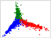
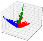
Figure 1: The orthogonality indicates a maximal separability among classes: subspace visualization of AWA2 on three learned random classes by the proposed method.
In ZSL/GZSL, since the trained model has no observation of any sample from unseen classes, the mapping function is inherently biased towards seen classes [Fu et al., 2015; Guo et al., 2023], i.e., the mapped features are usually overfitted to clusters near seen classes, hence can hardly infer to unseen classes with satisfactory performance. To relieve the domain-biased overfitting, especially for GZSL, existing methods usually resorted to learning more representative features having less gap between seen/unseen classes. Some widely used approaches include 1) visual-semantics alignment, for smooth knowledge transfer [Schonfeld et al., 2019; Guo and Guo, 2020]; 2) generative methods (i.e., synthesize mimic samples of unseen classes), for training a holistic model [Huang et al., 2019; Zhao et al., 2022]; and 3) fine-grained methods, for extracting more generalizable features [Huynh and Elhamifar, 2020; Guo et al., 2023].
Despite certain relief from the domain bias, we observe that existing methods, may in turn, inevitably incur the underfitting phenomenon on their trained models. For example, most GZSL models usually tend to obtain higher Harmonic Mean metrics [Xian et al., 2017] of the test accuracy. In other words, the recognition tasks for seen and unseen classes can suppress each other, yielding two mediocre results across seen/unseen classes. Hence, the training of ZSL/GZSL can easily fluctuate between over-/under-fittings and degrade the model's generalization ability.
Moreover, it can be noted that existing methods mostly rely on a series of complex deep models to extract and fuse comprehensive features for superior recognition [Xie et al., 2019; Huynh and Elhamifar, 2020; Wang et al., 2018; Guo et al., 2023]. As a result, such training and deployment can be costly in terms of both computing and memory overhead. In this regard, we make an assumption that ZSL/GZSL can be more favorable to a scenario associated with resource-constrained devices due to the low or even zero data requirements. Such a scenario can also well align with ubiquitous devices and data in real-world applications. However, as far as we know, nearly no research has investigated lightweight ZSL/GZSL models deployed on resourceconstrained devices.
In this paper, we suggest that the above generalization and lightweight requirements can be jointly achieved by our properly designed parsimonious yet efficient network refactoring framework, namely, ParsNets. Specifically, we utilize a set of base linear networks to estimate the nonlinear visualsemantics mapping function that usually involves complex deep models, wherein, each base linear network can correspond to different components of the semantic space shared by both seen and unseen classes. To encourage the learned features to be most discriminative from each other and generalizable to novel concepts, we enforce a low-rank structure to the features of data samples from the same class and a high-rank structure to the features of data samples from all different classes. Hence, intra-class samples can reside in the same linear subspace, and meanwhile, inter-class subspaces can be orthogonal to each other (i.e., Figure 1). Such constructed maximal margin geometry is expected to facilitate a smooth knowledge transfer between seen and unseen classes since no entanglement exists. Moreover, to further encourage the model's adaptability and counterbalance over-/underfittings, we employ a set of sample-wise indicators to select a sparse subset of these base linear networks to form a composite predictor for each sample, thus the global nonlinearity can be collapsed into sparse local linearities to further reduce the computing complexity. Our contributions are three-fold:
- We propose ParsNets, which is the first work that provides a parsimonious and on-device-friendly framework for ZSL/GZSL by refactoring the nonlinear large net-
work into a composition of simple local linear networks.
- We enforce maximal margin geometry on the learned features to maximize the model's discrimination and generalization ability, thus enabling a smooth knowledge transfer between seen and unseen classes.
- We provide detailed theoretical explanations on the rationality and implementation guarantee of ParsNets, which indicates its feasibility.
2 RelatedWork
2.1 Visual-Semantics Mapping in ZSL/GZSL
Existing ZSL/GZSL methods adopt three approaches to construct the visual-semantics mapping, including forward, reverse, and intermediate functions. Among them, forward mapping is the mainstream that maps samples from their visual features to the semantic space and computes their compatibilities with class-level semantic descriptions [Akata et al., 2015; Schonfeld et al., 2019]. Conversely, reverse mapping suggests that projecting semantic features into the visual space may decrease the feature variances [Zhang et al., 2017]. Diverging from direct mappings, intermediate functions explore metric networks to compute compatibilities of paired input visual and semantic features in an intermediate space [Sung et al., 2018]. However, it's noted that the above methods are mostly built upon deep models, which are all innately computational and memory-intensive frameworks. In this paper, we follow the forward mapping approach to implement the visual-semantics mapping function that aligns with most methods.
2.2 Domain-Bias Problem
In recent years, extensive efforts have been made to relieve the domain bias caused by the disjoint train (seen) and test (unseen) classes. For example, some methods tried to align the visual and semantic features within the visualsemantics mapping function to enable a smooth knowledge transfer [Zhang and Saligrama, 2015; Schonfeld et al., 2019; Guo and Guo, 2020]. Differently, some other methods proposed to synthesize mimical samples conditioned on unseen class semantic descriptors and jointly train a holistic model combined with seen class samples [Huang et al., 2019; Zhao et al., 2022; Feng et al., 2022]. In contrast, some recent methods focused on fine-grained elements or key points within samples to extract more generalizable features between seen/unseen classes [Xie et al., 2019; Huynh and Elhamifar, 2020; Guo et al., 2023]. Despite the relief from domain-biased overfitting, we observe that underfitting can inevitably arise and fluctuate the training towards mediocre convergence for both seen and unseen classes. This paper focuses on exploring a better balance between over- and underfittings by the proposed maximal margin geometry and network refactoring.
3 Methodology
3.1 Preliminaries
Given a dataset from seen domain DS = {xi, ayi , yi}Ni=1 that contains N labeled samples xi ∈ X S with seen class labels yi ∈ Y S . The task of GZSL is to construct a model trained on DS while can also generalize well to unseen domain DU = {(xu , ayu, yu ) | xu ∈ X U , yu ∈ Y U }, where X S ∩ X U = ϕ and Y S ∩ Y U = ϕ. To achieve this goal, a set of shared perclass semantic descriptors A = AS ∪ AU is further specified for seen classes (ay ∈ AS ) and unseen classes (ayu ∈ AU ), respectively, which are widely implemented by attributes or word vectors. Thus, the model can be formalized into training a parameterized mapping function f : X → A that maps a sample x from its original feature space X, e.g., visual space w.r.t. images, to the shared semantic space A as:
where L (·) minimizes the variance between mapped semantic features and ground-truth descriptors and φ (·) regularizes the network weight Θ, if needed. During inference, given a test sample xt , the recognition can be described as:
where Λ(·) is a similarity metric that searches the most closely related descriptor from A, whose class is then assigned to the sample. Notably, if the search scope is restricted to AU , the recognition becomes the classic ZSL.
3.2 Adaptive Composition of Linear Networks
To break the dependence on complex deep models, one possible solution is to use local linearities to estimate the global nonlinearity [Liu et al., 2018; Li et al., 2020]. In this paper, we apply a similar strategy to construct the visual-semantics mapping function. Concretely, we assume that a complex nonlinearly separable space can have sufficient linearly separable subspaces, and as such, we refactor the deep function f (·;Θ) into several base linear networks as:
where ΘTi x + bi (i = 1, 2, . . . ,K) are a set of base linear networks with trainable weight ΘTi that jointly estimate f(x), and bi denotes the bias constant vector. Such an estimation directly reduces the overhead in terms of both computing and memory with only limited accuracy loss [Oiwa and Fujimaki, 2014; Liu et al., 2018; Li et al., 2020].
Differently, in our method, we further utilize a set of associated indicators ξi(·), i.e.,
to adaptively select a subset of {ΘTi } to form a composite sample-wise semantic predictor f(x) | ξi(x) for each x. Such indicators are expected to be binary and sparse signals to fit with diverse samples in both visual and semantic spaces. Notably, the binarity can provide a gated functionality to active specific ΘTi , and the sparsity pushes the composite predictor to explore a better balance between over-/under-fittings due to sample-wise selection. Without loss of generality, given the ξi(·) (introduced in sect. Sample-Wise Indicators), we define one variable Φ(x) as:
where ΞT(x) = [ξ1(x), · · · , ξK(x)] and ⊗ denotes the Kronecker production, and denote the variable Θ as:
Thus, the composite semantic predictor in Eq. 3 can be rewritten as a regression form as:
Note that Eq. 7 can be significantly reduced to a lightweight model with the sparse binary signals from ΞT(x), wherein, only a few numbers of {ΘTi } are activated. In other words, the nonlinear model f(x) can collapse into a linear model at each point x and its nearby local field.
Mathematically, Eq. 7 can be solved efficiently by constructing a quadratic programming problem with the structural risk minimization as:
where ayl is the expected semantic descriptor, γl and γ ∗ l are slack variables, and C is a non-negative weight that penalizes the prediction error ϵ. Since the input dimension is usually large, we can consider its dual form. Specifically, we introduce Lagrange multipliers αl ≥ 0, µl ≥ 0, α∗ l ≥ 0, and µ∗l ≥ 0 to obtain the Lagrange function as:
It is easy to note that such a function can be solved by obtaining the saddle point ∂L ∂Θ = 0, ∂L ∂γl = 0, and ∂L ∂γ ∗ l = 0, and we can rewrite Eq. 8 as:
where T (xl, xj) is a constructed transformation function defined via Eq. 5 as:
Solving this problem and obtaining αl and α∗ l , the model in Eq. 3 can then be described as:
3.3 Sample-Wise Indicators
As to the associated indicators Ξ (x) in Eq. 4, we expect such signals can have the following properties: 1) discrimination, which can provide sufficient compositions of linear networks for diverse samples; and 2) sparsity and binarity, which activate only a small subset of base linear networks to form the composite predictor. Based on this guidance, our method employs a unsupervised linear encoder (W)-decoder (W′ ) network to preliminarily capture the intrinsic data structure:
wherein, the latent embedding E = WX is usually more representative compressed variables that can be potentially used to construct the indicators Ξ(x). In practice, Eq. 13 can be reformulated as ∥∥X-WTWX∥∥2 by using the tied weights [Ranzato et al., 2007], i.e., W′ = WT , where only W remains for estimation, hence reducing the complexity. Notably, the rationality can also be explained by the PCA equivalence of tying the weights [Vincent et al., 2010], whose orthogonality of the compressed space is more favorable.
Now we elaborate on the design of Ξ(x). Given the embedding Ex ∈ Rh of a sample x, we split it into a set of K components:
that correspond to K base linear networks. To determine the selection, we calculate the variance of each E(i) x to the mean value of Ex, i.e., denoted as Var(i) (E(i) x | µEx ). Then, we can rewrite the indicators of Eq. 4 to:
where each ξi(x) = Var(i) . The rationality lies in that, if the variance of E(i) x is large, then the latent variables are more significant compared with others. Finally, to achieve a sparse subset of base linear networks, we rank all variances and select top-k indicators ξi(x), i.e., k ≪ K, and set them to 1, which can activate the corresponding base linear networks in Eq. 3 with (ΘTi x + bi ) · 1. Meanwhile, the remaining indicators are set to 0 to omit these base linear networks.
It is noticed that the encoder W can be a pre-trained building block based on DS . In our method, on the one hand, it can be used to construct the sample-wise indicators, and meanwhile, on the other hand, we can also use the latent embedding E = WX as the initial features of the composite linear networks of Eq. 3.
3.4 Orthogonality and Low-Rankness
The proposed composite linear networks provide the guarantee of a parsimonious and on-device-friendly framework for our ParsNets. In this section, inspired by subspace transformation [Qiu and Sapiro, 2015], we enforce a maximal margin geometry on the mapped features, i.e., low-rank structure to intra-class features and high-rank structure to inter-class features, respectively, which further guarantees the model's generalization ability.
Concretely, without loss of generality, given the weight Θi of a linear network described in Eq. 3, we rewrite it as the matrix form as ΘTi X, where X = [x1 | x2 | · · · | xN] ∈ DS with each column xi ∈ Rd denoting a labeled sample from total ∣∣Y S ∣∣ seen classes. Let Xv denote the sample matrix extracted from the columns of X that belong to v-th class, we construct a minimization problem as:
where ∥·∥∗ is the nuclear norm which is a relaxation form of the non-differentiable rank function rank(·), i.e., ∥∥ΘTi Xv ∥∥∗ , ∥∥ΘTi X∥∥∗ ≈ rank(ΘTi Xv), rank(ΘTi X).
Notably, in Eq. 16, ∥∥ΘTi Xv ∥∥∗ minimizes the rank of the mapped feature matrix of each class, which can encourage intra-class samples to reside in the same linear subspace. Meanwhile, ∥∥ΘTi X∥∥∗ maximizes the rank of the mapped feature matrix of all classes, which can additionally encourage the aforementioned linear subspaces to be orthogonal from each other, thus maximizing the generalization ability. Moreover, ∥∥ΘTi ∥∥ = 1 is an extra regularization term, i.e., corresponds to φ (Θ) in Eq. 1, to avoid zero solution ΘTi = 0, and ⟨Θi,Θj⟩ = 0 pushes each linear network to be independent of each other.
Now, we prove that the global minimum of Eq. 16 can be reached as 0, when each Xv is orthogonal to the other.
Proposition 1. If Xv and Xv′ are orthogonal to each other, where ∀v, v′ ∈ [1,K] and v ̸= v′ , then Eq. 16 reaches the global minimum, i.e., Eq. 16=0.
To prove Proposition 1, we first present two theorems, i.e., Theorem 1 and Theorem 2.
Theorem 1. Let M and N be matrices that have the same row dimensions, and let [M,N] be the concatenation of M and N, we have:∥[M, N]∥∗ ≤ ∥M∥∗ + ∥N∥∗ . (17)
Proof of Theorem 1. It can be proved easily via:
Theorem 2. Let M and N be matrices that have the same row dimensions, and let [M,N] be the concatenation of M and N, we have:∥[M, N]∥∗ = ∥M∥∗ + ∥N∥∗ , (19)
when M and N are column-wise orthogonal.
Proof of Theorem 2. We apply the singular value decomposition to M and N as:
where ∑M and ∑N contain non-zero singular values, then we can have:
Given that M and N are column-wise orthogonal, i.e., UM1 ′UN1 = 0, then Eq. 21 can be rewritten as:
Then we can have:
Since the nuclear norm ∥M∥∗ equals the sum of the square root of the singular values of MM′ , so we can have ∥[M,N]∥∗ = ∥M∥∗ + ∥N∥∗ that proves Eq. 19.
Proof of Proposition 1. Theorem 1 and Theorem 2 can obviously be extended to multiple matrices. As a result, for Eq. 16, we have:
Based on Theorem 2 and Eq. 24, the minimization problem described in Eq. 16 can achieve the global minimum of 0, if the column spaces of all pairs of matrices are orthogonal.
4 Experiments
4.1 Experimental Setup
Dataset. We evaluate our ParsNets on four widely used ZSL/GZSL benchmark datasets, including AWA2 [Xian et al., 2018a], CUB-200 [Wah et al., 2011], SUN [Patterson et al., 2014], and aPY [Farhadi et al., 2009]. As to the splitting strategy of seen and unseen classes for each dataset, we and all involved competitors strictly follow [Xian et al., 2018a], which is the most adopted benchmark splitting for ZSL/GZSL, to ensure a fair comparison.
Evaluation Metrics. Two different scenarios are considered in our experiments, including the classic ZSL and GZSL. For ZSL, the recognition only searches the test samples from unseen classes and reports the multi-way classification accuracy as in previous works for our method and each involved competitor. Differently, for GZSL, we compute the average per-class prediction accuracy on test samples from unseen classes (U) and seen classes (S), respectively, and report the Harmonic Mean calculated by H = (2 × U × S) / (U + S) to quantify the aggregate performance across both seen and unseen classes. As to the competitors, we select representative deep learning-based ZSL/GZSL methods based on the following criteria: 1) formally published in the most recent years; 2) covered a wide range of models; 3) all of them clearly represented the state-of-the-art.
Implementation. We implement the proposed ParsNets on Raspberry Pi 4B 1 , which is a widely used low-cost edge device platform equipped with ARM Cortex-A72 CPU and 4GB RAM. Similar to the server-based computing architecture, the edge platform is installed with Ubuntu 20.10, Miniconda3, and PyTorch 1.8.0. that can support most modeling frameworks. To construct the ParsNets, we use the singlelayer neural network with ReLU activation function for each of the base linear networks in Eq. 3, and the total number of the networks K is empirically set as 200 for all datasets. As to the sample-wise indicators in Eq. 15, we rank all variances and then enable k ranges in {10, 20, 30, 40, 80, 120, 160, 200}, which corresponds to {5%, 10%, 15%, 20%, 40%, 60%, 80%, 100%} of the total base linear networks that have been activated during training. For the visual representation, we use the 2048-dimensional visual features extracted from ResNet for each input sample, which is common practice for most methods. Notably, the other competitors are all implemented and running on server-based computers along with powerful GPUs and large storage, further highlighting the ondevice-friendly functionality of our method.
4.2 Comparison of ZSL Performance
We compare the proposed ParsNets with 16 state-of-the-art deep learning-based competitors in the classic ZSL scenario and report the multi-way classification accuracy in Table 1. It can be observed from the results that our method outperforms most deep learning-based competitors on all datasets. For example, DGZ [Chen et al., 2023] and TDCSS [Feng et al., 2022] are the most two powerful generative model-based ZSL competitors that can achieve 80.1% and 61.1% recognition accuracy on CUB-200. In contrast, despite as a non-deep method, our method obtains 0.2% and 19.2% higher performance with much lower computing cost. On the other hand, as a complex graph fine-grained method that utilized powerful GNNs as the sample representation, GKU [Guo et al., 2023] achieves 76.9% on CUB-200. In contrast, our method obtains a much better performance of 80.3% with/on only the resource-constrained device.
4.3 Comparison of GZSL Performance
As shown in Table 2, we compare the proposed ParsNets with 16 state-of-the-art deep learning-based competitors in the GZSL scenario and report the average per-class prediction accuracy on unseen classes (U), seen classes (S), and their Harmonic Mean (H). We can observe that our method also constantly outperforms other deep learning-based competitors by even improved margins than that of the ZSL scenario on all datasets. Specifically, in GZSL, most competitors can hardly achieve balanced performance in both seen and unseen classes due to the domain-biased over-/underfittings problem. For example, in Zhu et al. [Zhu et al., 2019] and APNet [Liu et al., 2020], there exist 49.5% and 42.0% margins between the accuracy of seen and unseen classes in AWA2 and aPY, respectively, thus the overall performance, i.e, Harmonic Mean, is significantly poor for real-world application. Moreover, even some of the most powerful competitors such as PSVMA [Liu et al., 2023] and DGZ [Chen et al., 2023] can still have a nonnegligible margin, i.e., 16.4% and 12.3% in SUN and AWA2, respectively. In contrast, due to the utilization of the proposed sample-wise composite semantic predictor and the constructed maximal margin geometry, our method can significantly relieve the domain-biased over-/under-fittings problem and obtain a more balanced performance in both seen and unseen classes.
1 www.raspberrypi.com/products/raspberry-pi-4-model-b
| Method | Venue | AWA2 | CUB-200 | SUN | aPY |
|---|---|---|---|---|---|
| SE-ZSL [Kumar Verma et al., 2018] f-CLSWGAN [Xian et al., 2018b] Zhu et al. [Zhu et al., 2019] AREN [Xie et al., 2019] APNet [Liu et al., 2020] RGEN [Xie et al., 2020] OCD-CVAE [Keshari et al., 2020] DAZLE [Huynh and Elhamifar, LsrGAN [Vyas et al., 2020] APN [Xu et al., 2020] HSVA [Chen et al., 2021a] VGSE [Xu et al., 2022] TDCSS [Feng et al., 2022] PSVMA [Liu et al., 2023] GKU [Guo et al., 2023] DGZ [Chen et al., 2023] | CVPR ′ 18 CVPR ′ 18 NeurIPS ′ CVPR ′ 19 AAAI ′ 20 ECCV ′ 20 CVPR ′ 20 CVPR ′ 20 ECCV ′ 20 NeurIPS ′ NeurIPS ′ CVPR ′ 22 CVPR ′ 22 CVPR ′ 23 AAAI ′ 23 AAAI ′ 23 | 80.8 - | 60.3 57.3 70.5 70.7 57.7 76.1 60.8 64.1 60.3 72.0 62.8 28.9 61.1 72.9 76.9 80.1 | 64.5 60.8 - 61.7 62.3 63.8 68.9 62.5 62.5 61.6 63.8 38.1 - 66.5 - 65.4 | 39.8 - - - - - - - - - - |
| 68.2 | |||||
| 19 | 83.5 | ||||
| 67.9 | 44.1 | ||||
| 68.0 | 41.3 | ||||
| 73.6 | 44.4 | ||||
| 81.7 | |||||
| 2020] | 75.2 | ||||
| 66.4 | |||||
| 20 | 68.4 | ||||
| 21 | 70.6 | ||||
| 64.0 | |||||
| 71.2 | |||||
| 79.4 | 45.9 | ||||
| 74.0 | 46.6 | ||||
| ParsNets (ours) | Proposed | 82.6 | 80.3 | 70.2 | 48.7 |
4.4 Complexity
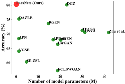
In Figure 2, we briefly compare the model complexity between the proposed ParsNets and some existing deep models. Specifically, we record the number of model parameters, i.e., denoted as 'M', and the ZSL accuracy (%) on the CUB-200 dataset one by one, and visualize their comparison results. We can observe that our ParsNets, i.e., denoted in 'Red', can obtain the best accuracy with the least number of parameters against all deep models, which is a hardware-level guarantee for the on-device utilization.
4.5 Mapping Robustness
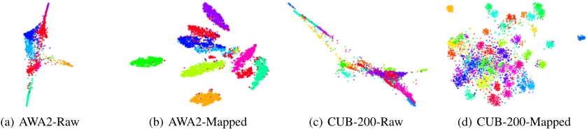
To further demonstrate the effectiveness of our method in relieving the domain-biased over-/under-fittings problems, we visualize the raw and mapped features of samples from test unseen classes of AWA2 (10 unseens) and CUB-200 (50 unseens), respectively, using t-SNE [Van der Maaten and Hinton, 2008] in Figure 3. It can be observed that we can pose more subspaces between different classes with the obtained mapped features than the results with raw features. Specifically, Figure 3(a) and Figure 3(c) are the visualizations of raw features of AWA2 and CUB-200, respectively, where most classes are clustered in panhandle subspaces. In contrast, Figure 3(b) and Figure 3(d) are the visualizations of mapped features of AWA2 and CUB-200, respectively, by reusing the trained model based on only seen classes. It is obvious that the mapped feature space results in more subspaces for different classes, thus our method can be more separable and robust across both seen and unseen classes.
4.6 Ablation Study
We consider three scenarios to verify the effectiveness of the parsimonious network design in ZSL performance, including 1) only the sample-wise composite linear networks (SCLN) are used; 2) only the maximal margin geometry (MMG) is used (with all base linear networks activated); and 3) full ParsNets with both SCLN and MMG. The results are demonstrated in Table 3. We can observe that by using only SCLN or MMG separately, the performance is mediocre across all datasets. However, if both SCLN and MMG are used to form the ParsNets, our recognition performance is significantly improved with a large margin of 15.4% in AWA2, 21.5% in CUB-200, 18.8% in SUN, and 10.4% in aPY. Such an improvement fully demonstrates the effectiveness and rationality of our method.
| Method | Venue | AWA2 | CUB-200 | SUN | aPY | ||||||||
|---|---|---|---|---|---|---|---|---|---|---|---|---|---|
| U | S | H | U | S | H | U | S | H | U | S | H | ||
| f-CLSWGAN [Xian et al., 2018b] SE-GZSL [Kumar Verma et al., Zhu et al. [Zhu et al., 2019] AREN [Xie et al., 2019] LsrGAN [Vyas et al., 2020] DAZLE [Huynh and Elhamifar, OCD-CVAE [Keshari et al., 2020] RGEN [Xie et al., 2020] APNet [Liu et al., 2020] HSVA [Chen et al., 2021a] TDCSS [Feng et al., 2022] VGSE [Xu et al., 2022] GKU [Guo et al., 2023] DGZ [Chen et al., 2023] VS-Boost [Li et al., 2023] | CVPR ′ 18 | 57.9 58.3 - | 61.4 68.1 87.1 | 59.6 62.8 52.5 | 43.7 | 57.7 | 49.7 | 42.6 | 36.6 | 39.4 | - | - | - |
| 2018] | CVPR ′ 18 | 41.5 | 53.3 | 46.7 | 40.9 | 30.5 | 34.9 | - | - | - | |||
| NeurIPS ′ 19 | 37.6 | 36.7 | 71.3 | 48.5 | - | - | - | - | - | - | |||
| CVPR ′ 19 | 54.7 | 79.1 | 64.7 | 63.2 | 69.0 | 66.0 | 40.3 | 32.3 | 35.9 | 30.0 | 47.9 | 36.9 | |
| ECCV ′ 20 | 54.6 | 74.6 | 63.0 | 48.1 | 59.1 | 53.0 | 44.8 | 37.7 | 40.9 | - | - | - | |
| 2020] | CVPR ′ 20 | 75.7 | 60.3 | 67.1 | 59.6 | 56.7 | 58.1 | 24.3 | 52.3 | 33.2 | - | - | - |
| CVPR ′ 20 | 59.5 | 73.4 | 65.7 | 44.8 | 59.9 | 51.3 | 44.8 | 42.9 | 43.8 | - | - | - | |
| ECCV ′ 20 | 67.1 | 76.5 | 71.5 | 60.0 | 73.5 | 66.1 | 44.0 | 31.7 | 36.8 | 30.4 | 48.1 | 37.2 | |
| AAAI ′ 20 | 83.9 | 54.8 | 66.4 | 55.9 | 48.1 | 51.7 | 40.6 | 35.4 | 37.8 | 74.7 | 32.7 | 45.5 | |
| NeurIPS ′ 21 | 56.7 | 79.8 | 66.3 | 52.7 | 58.3 | 55.3 | 48.6 | 39.0 | 43.3 | - | - | - | |
| CVPR ′ 22 | 59.2 | 74.9 | 66.1 | 44.2 | 62.8 | 51.9 | - | - | - | - | - | - | |
| CVPR ′ 22 | 51.2 | 81.8 | 63.0 | 21.9 | 45.5 | 29.5 | 24.1 | 31.8 | 27.4 | - | - | - | |
| AAAI ′ 23 | - | - | 52.3 | 71.1 | 60.3 | - | - | - | - | - | - | ||
| AAAI ′ 23 | 65.9 | 78.2 | 71.5 | 71.4 | 64.8 | 68.0 | 49.9 | 37.6 | 42.8 | 38.0 | 63.5 | 47.6 | |
| IJCAI ′ 23 | 67.9 | 81.6 | 74.1 | 68.0 | 68.7 | 68.4 | 49.2 | 37.4 | 42.5 | 49.8 | 69.6 | 58.1 | |
| PSVMA [Liu et al., 2023] | CVPR ′ 23 | 73.6 | 77.3 | 75.4 | 70.1 | 77.8 | 73.8 | 61.7 | 45.3 | 52.3 | - | - | - |
| ParsNets (ours) | Proposed | 77.6 | 81.4 | 79.5 | 72.8 | 79.4 | 76.0 | 57.2 | 49.5 | 53.1 | 42.3 | 68.6 | 52.3 |
| Module | AWA3 | CUB-200 | SUN | aPY | |
|---|---|---|---|---|---|
| SCLN | MMG | (%) | (%) | (%) | (%) |
| ✓ | 67.2 | 58.8 | 51.4 | 38.3 | |
| ✓ | 69.5 | 67.2 | 55.2 | 40.1 | |
| ✓ | ✓ | 82.6 | 80.3 | 70.2 | 48.7 |
4.7 Sparseness Analysis
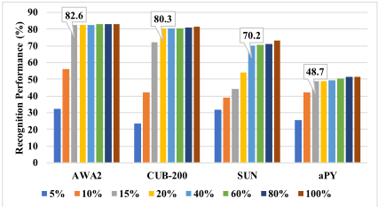
The sample-wise indicators are another important criterion in our method, where we need to select top-k indicators to activate k (out of total K) base linear networks to form the sparse composite linear networks for each sample. We rank all variances in Eq. 15 and then enable k ranges in {10, 20, 30, 40, 80, 120, 160, 200} during training, which corresponds to a sparsity of {5%, 10%, 15%, 20%, 40%, 60%, 80%, 100%} out of the total number of base linear networks. We repeat the running on all datasets and record the ZSL recognition accuracy of each sparsity in Figure 4. It can be observed that as the number of base linear networks increases, the accuracy gradually improves at the very beginning phase. Soon, it reaches a stable phase where we can explore a trade-off between recognition accuracy and sparsity for each dataset. Specifically, we set k = 30 (15%) for AWA2, k = 40 (20%) for CUB-200, k = 80 (40%) for SUN, and k = 30 (15%) for aPY.
5 Conclusion
We proposed ParsNets, which is a novel parsimonious yet efficient ZSL/GZSL framework with on-device friendly properties. Its gist, as well as our novelty, mainly lies in three aspects: 1) the utilization of simple local linear networks to estimate nonlinear large visual-semantics mapping function; 2) the maximal margin geometry-enabled orthogonal subspaces to smooth out the seen/unseen knowledge transfer; and 3) the sample-wise indicators to enable sparse compositions of base linear networks. Experimental results verified the effectiveness of our method.
Acknowledgments
This research was supported by funding from the Hong Kong RGC General Research Fund (grant numbers 152211/23E and 15216424/24E), the National Natural Science Foundation of China (grant number 62102327), and the PolyU Internal Fund (grant number P0043932). This research was also supported by NVIDIA AI Technology Center (NVAITC).
@inproceedings{ijcai2024p449,
  title     = {ParsNets: A Parsimonious Composition of Orthogonal and Low-Rank Linear Networks for Zero-Shot Learning},
  author    = {Guo, Jingcai and Zhou, Qihua and Lu, Xiaocheng and Li, Ruibin and Liu, Ziming and Zhang, Jie and Han, Bo and Chen, Junyang and Xie, Xin and Guo, Song},
  booktitle = {Proceedings of the Thirty-Third International Joint Conference on
               Artificial Intelligence, {IJCAI-24}},
  publisher = {International Joint Conferences on Artificial Intelligence Organization},
  editor    = {Kate Larson},
  pages     = {4062--4070},
  year      = {2024},
  month     = {8},
  note      = {Main Track},
  doi       = {10.24963/ijcai.2024/449},
  url       = {https://doi.org/10.24963/ijcai.2024/449},
}
TY - CPAPER TI - ParsNets: A Parsimonious Composition of Orthogonal and Low-Rank Linear Networks for Zero-Shot Learning AU - Guo, Jingcai AU - Zhou, Qihua AU - Lu, Xiaocheng AU - Li, Ruibin AU - Liu, Ziming AU - Zhang, Jie AU - Han, Bo AU - Chen, Junyang AU - Xie, Xin AU - Guo, Song T2 - Proceedings of the Thirty-Third International Joint Conference on Artificial Intelligence, IJCAI-24 PB - International Joint Conferences on Artificial Intelligence Organization PY - 2024 SP - 4062 EP - 4070 DO - 10.24963/ijcai.2024/449 UR - https://doi.org/10.24963/ijcai.2024/449 ER -Copied
Machine-readable versions of this paper, for tools and AI agents:





