
Deep Multi-Dimensional Classification with Pairwise Dimension-Specific Features
Proceedings of the Thirty-Third International Joint Conference on Artificial Intelligence. Main Track. Pages 4183-4191.
https://doi.org/10.24963/ijcai.2024/462
Keywords
- Machine Learning: ML: Multi-label learning
- Machine Learning: ML: Classification
Abstract
In multi-dimensional classification (MDC), each instance is associated with multiple class variables characterizing the semantics of objects from different dimensions. To consider the dependencies among class variables and the specific characteristics contained in different semantic dimensions, a novel deep MDC approach named PIST is proposed to jointly deal with the two issues via learning pairwise dimension-specific features. Specifically, PIST conducts pairwise grouping to model the dependencies between each pair of class variables, which are more reliable with limited training samples. For extracting pairwise dimension-specific features, PIST weights the feature embedding with a feature importance vector, which is learned via utilizing a global loss measurement based on intra-class and inter-class covariance. Final prediction w.r.t. each dimension is determined by combining the joint probabilities related to this dimension. Comparative studies with eleven real-world MDC data sets clearly validate the effectiveness of the proposed approach.
- [Bielza et al., 2011] Concha Bielza, Guangdi Li, and Pedro Larrañaga. Multi-dimensional classification with Bayesian networks. International Journal of Approximate Reason- ing, 52(6):705-727, 2011.
- [Borchani et al., 2013] Hanen Borchani, Concha Bielza, Carlos Toro, and Pedro Larrañaga. Predicting human im- munodeficiency virus inhibitors using multi-dimensional Bayesian network classifiers. Artificial Intelligence in Medicine, 57(3):219-229, 2013.
- [Chang and Lin, 2011] Chih-Chung Chang and Chih-Jen Lin. LIBSVM: A library for support vector machines. ACM Trans. Intell. Syst. Technol., 2(3):27:1-27:27, 2011.
- [Demšar, 2006] Janez Demšar. Statistical comparisons of classifiers over multiple data sets. Journal of Machine Learning Research, 7:1-30, 2006.
- [Fernandez Gonzalez et al., 2015] Pablo Fernandez Gonza- lez, Pedro Maria Larrañaga Mugica, and Maria Concep- cion Bielza Lozoya. Multidimensional classifiers for neu- roanatomical data. In Proceedings of the ICML Workshop on Statistics, Machine Learning and Neuroscience, pages 1-6, Lille, France, 2015.
- [Gil-Begue et al., 2021] Santiago Gil-Begue, Concha Bielza, and Pedro Larrañaga. Multi-dimensional Bayesian network classifiers: A survey. Artificial Intelligence Review, 54(1):519-559, 2021.
- [Jia and Zhang, 2020a] Bin-Bin Jia and Min-Ling Zhang. Multi-dimensional classification via kNN feature augmen- tation. Pattern Recognition, 106:107423, 2020.
- [Jia and Zhang, 2020b] Bin-Bin Jia and Min-Ling Zhang. Multi-dimensional classification via stacked dependency exploitation. Science China Information Science, 63(12):222102, 2020.
- [Jia and Zhang, 2021a] Bin-Bin Jia and Min-Ling Zhang. MDKNN: An instance-based approach for multi- dimensional classification. In Proceedings of the 25th International Conference on Pattern Recognition, pages 126-133, Virtual Event / Milan, Italy, 2021.
- [Jia and Zhang, 2021b] Bin-Bin Jia and Min-Ling Zhang. Multi-dimensional classification via sparse label encoding. In Proceedings of the 38th International Conference on Machine Learning, pages 4917-4926, Virtual Event, 2021.
- [Jia and Zhang, 2022] Bin-Bin Jia and Min-Ling Zhang. Multi-dimensional classification via selective feature aug- mentation. Machine Intelligence Research, 19(1):38-51, 2022.
- [Jia et al., 2023] Bin-Bin Jia, Jun-Ying Liu, Jun-Yi Hang, and Min-Ling Zhang. Learning label-specific features for decomposition-based multi-class classification. Frontiers of Computer Science, 17(6):176348, 2023.
- [Lertnattee and Theeramunkong, 2004] Verayuth Lertnattee and Thanaruk Theeramunkong. Multidimensional text classification for drug information. IEEE Transactions on Information Technology in Biomedicine, 8(3):306-312, 2004.
- [Lian et al., 2020] Zheng Lian, Ya Li, Jianhua Tao, Jian Huang, and Mingyue Niu. Expression analysis based on face regions in real-world conditions. International Jour- nal of Automation and Computing, 17(1):96-107, 2020.
- [Ma and Chen, 2018] Zhongchen Ma and Songcan Chen. Multi-dimensional classification via a metric approach. Neurocomputing, 275:1121-1131, 2018.
- [Read et al., 2014a] Jesse Read, Concha Bielza, and Pedro Larrañaga. Multi-dimensional classification with super- classes. IEEE Transactions on Knowledge and Data Engi- neering, 26(7):1720-1733, 2014.
- [Read et al., 2014b] Jesse Read, Luca Martino, and David Luengo. Efficient monte carlo methods for multi- dimensional learning with classifier chains. Pattern Recognition, 47(3):1535-1546, 2014.
- [Saleh and Li, 2023] Ahmed Abdelfattah Saleh and Weigang Li. Deep self-organizing cube: A novel multi-dimensional classifier for multiple output learning. Expert Systems with Applications, 230:120627, 2023.
- [Shatkay et al., 2008] Hagit Shatkay, Fengxia Pan, Andrey Rzhetsky, and W. John Wilbur. Multi-dimensional clas- sification of biomedical text: Toward automated, practical provision of high-utility text to diverse users. Bioinformat- ics, 24(18):2086-2093, 2008.
- [Shi et al., 2025] Yi Shi, Han-Jia Ye, Dong-Liang Man, Xiao-Xu Han, De-Chuan Zhan, and Yuan Jiang. Revisiting multi-dimensional classification from a dimension-wise perspective. Frontiers of Computer Science, 19(1):191304, 2025.
- [Song et al., 2018] Lingyun Song, Jun Liu, Buyue Qian, Mingxuan Sun, Kuan Yang, Meng Sun, and Samar Ab- bas. A deep multi-modal CNN for multi-instance multi- label image classification. IEEE Transactions on Image Processing, 27(12):6025-6038, 2018.
- [Srivastava et al., 2014] Nitish Srivastava, Geoffrey Hinton, Alex Krizhevsky, Ilya Sutskever, and Ruslan Salakhutdi- nov. Dropout: a simple way to prevent neural networks from overfitting. Journal of Machine Learning Research, 15(1):1929-1958, 2014.
- [Tang et al., 2024] Jun Tang, Wenhui Chen, Ke Wang, Yan Zhang, and Dong Liang. Probability-based label enhance- ment for multi-dimensional classification. Information Sciences, 653:119790, 2024.
- [Wang et al., 2016] Jiang Wang, Yi Yang, Junhua Mao, Zhi- heng Huang, Chang Huang, and Wei Xu. CNN-RNN: A unified framework for multi-label image classification. In Proceedings of the 27th IEEE Conference on Computer Vi- sion and Pattern Recognition, pages 2285-2294, Las Ve- gas, NV, USA, 2016.
- [Wang et al., 2020] Haobo Wang, Chen Chen, Weiwei Liu, Ke Chen, Tianlei Hu, and Gang Chen. Incorporat- ing label embedding and feature augmentation for multi- dimensional classification. In Proceedings of the 34th AAAI Conference on Artificial Intelligence, pages 6178- 6185, New York, NY, USA, 2020.
- [Yeh et al., 2017] Chih-Kuan Yeh, Wei-Chieh Wu, Wei-Jen Ko, and Yu-Chiang Frank Wang. Learning deep latent space for multi-label classification. In Proceedings of the 31st AAAI Conference on Artificial Intelligence, pages 2838-2844, San Francisco, CA, USA, 2017.
- [Zaragoza et al., 2011] Julio H. Zaragoza, Luis Enrique Su- car, Eduardo F. Morales, Concha Bielza, and Pedro Larrañaga. Bayesian chain classifiers for multidimen- sional classification. In Proceedings of the 22nd Inter- national Joint Conference on Artificial Intelligence, pages 2192-2197, Barcelona, Catalonia, Spain, 2011.
- [Zhang et al., 2018] Min-Ling Zhang, Yu-Kun Li, Xu-Ying Liu, and Xin Geng. Binary relevance for multi-label learning: An overview. Frontiers of Computer Science, 12(2):191-202, 2018.
- [Zhang et al., 2022] Wenbo Zhang, Yunhao Gou, Yuepeng Jiang, and Yu Zhang. Adversarial VAE with normalizing flows for multi-dimensional classification. In Proceedings of the 5th Chinese Conference on Pattern Recognition and Computer Vision, pages 205-219, Shenzhen, China, 2022.
- [Zhang et al., 2023] Bo Zhang, Jun Zhu, and Hang Su. To- ward the third generation artificial intelligence. Science China Information Sciences, 66(2):121101, 2023.
- [Zhu et al., 2016] Mingmin Zhu, Sanyang Liu, and Jiewei Jiang. A hybrid method for learning multi-dimensional bayesian network classifiers based on an optimization model. Applied Intelligence, 44(1):123-148, 2016.
References were extracted automatically from the PDF and may contain errors.
Full text extracted automatically from the PDF; figures, tables and equations may differ. The PDF is the version of record.
1 Introduction
In multi-dimensional classification (MDC), each object is represented by a single instance while associated with multiple class variables. Here, each class variable corresponds to one label space characterizing the rich semantics of objects from some specific dimension. Take landscape paintings classification as an example, each picture can be classified from time dimension (with possible labels morning, afternoon, night, etc.), from whether dimension (with possible labels sunny, rainy, cloudy, etc.), and from scene dimension (with possible labels desert, mountain, grass, etc.). Specifically, the needs of learning fromMDC objects widely exist in diverse real-world applications, including text mining [Lertnattee and Theeramunkong, 2004; Shatkay et al., 2008], computer vision [Song et al., 2018; Lian et al., 2020; Shi et al., 2025], bioinformatics [Borchani et al., 2013; Fernandez Gonzalez et al., 2015], etc.
∗Corresponding author
Formally speaking, given a feature space X = Rd and an output space Y = C1 × C2 × · · · × Cq corresponding to the Cartesian product of q label spaces, each label space Cj = {cj1 , cj2 , . . . , cjKj } includes Kj possible labels (1 ≤ j ≤ q) to characterize the semantics along one dimension. Let D = {(xi, yi)|1 ≤ i ≤ m} be the training set and each sample (xi, yi) corresponds to a d-dimensional feature vector xi = [xi1, xi2, . . . , xid]T ∈ X associated with a q-dimensional label vector yi = [yi1, yi2, . . . , yiq]T ∈ Y. Given an unseen instance x∗, the task of MDC is to learn a mapping function f : X ↦→ Y from the training set D which can return a proper label vector f(x∗).
One popular solution to MDC tasks is to independently deal with each dimension as a traditional multi-class classification problem. Nonetheless, this strategy completely ignores the dependencies among class variables and then the performance of the induced predictive model might degenerate. To tackle this issue, existing MDC approaches are designed to consider class dependencies in either explicit manner with some structures (e.g., directed acyclic graph [Bielza et al., 2011; Gil-Begue et al., 2021], chaining order [Zaragoza et al., 2011] and pairwise interaction [Jia and Zhang, 2020b]) or in implicit manner via manipulating feature space [Jia and Zhang, 2020a; Jia and Zhang, 2022] or label space [Jia and Zhang, 2021b; Tang et al., 2024].
Although these existing approaches have successfully considered class dependencies, they might obtain suboptimal performances since the predictive models for different dimensions are induced based on the same feature space [Jia et al., 2023]. However, different semantics in each dimension might prefer different feature characteristics. Take the aforementioned landscape painting as an example, the level of luminance would be preferred in discriminating labels in time dimension; abrupt color changes are more likely to reveal the labels in scene dimension and the upper part of a picture is supposed to be more related to whether dimension. Moreover, samples belonging to the same class should be similar in the feature space generally, but it is very common that two MDC samples belong to the same class in one dimension while different classes in another dimension.
To consider the specific characteristics contained in different semantic dimensions as well as the dependencies among class variables, we propose a novel MDC approach named PIST (i.e., Pairwise dImension-Specific feaTures) based on deep learning techniques. Specifically, PIST aims to model class dependencies between each pair of class variables via pairwise grouping. Firstly, to construct pairwise dimensional embeddings, a combinatorial encoding procedure is conducted for pairwise class variables via optimizing the intraclass and inter-class covariance. Then an element-wise selection mechanism is used to extract pairwise dimension-specific features, which are considered better capturing the correlation between feature space and heterogeneous label semantics in respective dimension pairs. Finally, joint probabilities predicted by pairwise neural networks are integrated to accomplish the final discrimination collectively. To the best of our knowledge, PIST serves as the first attempt towards learning dimension-specific features as well as considering class dependencies. Comprehensive experiments on eleven benchmark data sets show that PIST performs better than existing well-established MDC approaches.
The rest of this paper is organized as follows. Firstly, Section 2 briefly reviews related works. Then Section 3 presents the proposed PIST approach at length. After that, Section 4 reports the results of empirical studies over a wide range of MDC data sets. Finally, Section 5 concludes this paper.
2 RelatedWork
On one hand, MDC can be regarded as a set of multi-class classification problems, one per dimension. Thus, we can solve the MDC problem by learning an independent multiclass classifier for each dimension, which is known as binary relevance (BR) [Zhang et al., 2018] but ignores all possible class dependencies. To exploit class dependencies among dimensions, on the other hand, one straightforward strategy is to regard each distinct label combination as a new class, which is known as class powerset (CP). However, the combinatorial nature of CP induces high complexity and is also prone to class-imbalance and overfitting problem. According to the strategy of dependency modeling, existing MDC works can be roughly categorized into two categories, including explicit and implicit dependency modeling methods.
The MDC methods of explicit category attempt to model class dependencies with some explicit structures. Chainingbased classifiers improve BR by learning a chain of multi-class classifiers, where subsequent classifiers on the chain will augment predictions of preceding one as features [Zaragoza et al., 2011; Read et al., 2014b]. Multidimensional Bayesian classifiers construct directed acyclic graph over class variable to explicitly consider the class dependencies [Bielza et al., 2011; Gil-Begue et al., 2021]. Generally, the dependencies among many class variables are hard to model due to limited samples in training set. SEEM [Jia and Zhang, 2020b] and MDKNN [Jia and Zhang, 2021a] suggest that pairwise dependencies can be modeled more reliably than modeling the dependencies among all class variables.
The MDC methods of implicit category attempt to transform the original MDC problem into a new one without some explicit dependency modeling mechanism in the transformation procedure. gMML [Ma and Chen, 2018] transforms the original categorical output space into a binary one and then induce the predictive model based on metric learning.
SLEM [Jia and Zhang, 2021b] encodes the original class vectors into real-valued ones and decodes the predicted class vectors over the outputs of learned multi-output regression model. To extract more powerful features, KRAM [Jia and Zhang, 2020a] manipulates the feature space via utilizing kNN information to enrich the original feature space.
LEFA [Wang et al., 2020] is the first MDC approach that utilizes deep learning techniques. It learns an augmented feature vector for each instance via assuming that the representations of features and labels should be aligned in some latent space. ADVAE-FLOW [Zhang et al., 2022] encodes both feature and class variables to probabilistic latent spaces by normalizing flows, in which the one-hot representation for the label vectors w.r.t. different dimensions are directly stacked. DSOC [Saleh and Li, 2023] is formed of multiple neural networks and a hypercube classifier, where the former are responsible for feature selection and the latter aims to accommodate the model for rare sample classification.
However, all these works only aim to consider class dependencies but cannot consider the specific characteristics contained in different semantic dimensions. In the next section, we will present the technical details of the proposed PIST approach, which considers not only class dependencies but also pairwise dimension-specific characteristics.
3 The PIST Approach
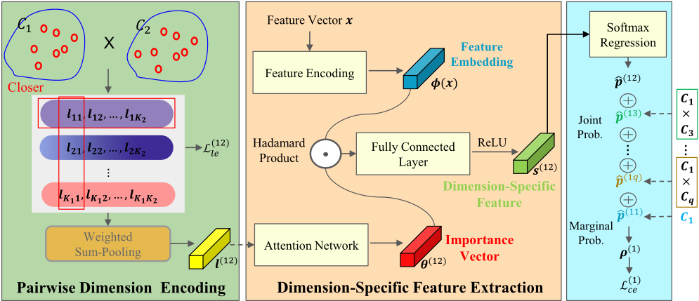
As shown in Figure 1, PIST includes two key modules: pairwise dimension encoding and dimension-specific feature extraction. Briefly, a weighted sum-pooling is conducted to obtain pairwise dimension embeddings in the first module and the outputs will further guide the dimension-specific feature extraction in the second module. The final classification is enabled by the returned probabilities of softmax regression.
3.1 Pairwise Dimension Encoding
To consider pairwise interactions, PIST considers each pair of dimensions as an entirety. Without loss of generality, we will carry out the following discussions in the case of C1 and C2. To extract dimension-specific features for this dimension pair, PIST learns a corresponding pairwise dimension embedding with a weighted sum-pooling as follows:
where fa1a2 is the number of samples labeled by c1a1 and c2a2 in the training set and la1a2 ∈ Rt is a latent label embedding vector related to c1a1 and c2a2 . Here, t is a hyper-parameter to be set (cf. Section 4.3 for further discussions).
For each component la1a2 in Eq.(1), a natural cluster assumption is that la11, la12, . . . , la1K2 are close to each other and far from l˜a11, l˜a12, . . . , l˜a1K2 where a1 ∈ {1, 2, . . . ,K1} and ˜a1 ∈ {1, 2, . . . ,K1} \ {a1}. For this purpose, good embeddings la1a2 should minimize the intra-class covariance and maximize inter-class covariance, which can be implemented via minimizing the following objective L(12) le-part1 :
where ¯ la1 = 1 K2 ∑K2 a2=1 la1a2 is the intra-class mean and ¯ l = 1 K1K2 ∑K1 a1=1 ∑K2 a2=1 la1a2 is the global mean.
It is worth noting that the above discussions on similarity of latent label embeddings have another 'dual' form with an exchange of subscript a1 and a2. Then another objective L(12) le-part2 is as follows:
where ¯ l′a2 = 1 K1 ∑K1 a1=1 la1a2 is the 'dual' intra-class mean. By combining the two above objectives together, the final label embedding loss L(12) le w.r.t. C1 and C2 can be defined as follows:
3.2 Dimension-Specific Feature Extraction
For each example x, numerous early works [Yeh et al., 2017; Wang et al., 2016; Zhang et al., 2023] have proved that it is significant to exploit powerful feature embeddings in latent spaces. Thus we firstly encode x into a latent space based on neural networks which is denoted by ϕ(x) ∈ Rd′ . To extract pairwise dimension-specific feature, decode l(12) into a feature importance vector with an attention network:
where θ(12) , bl ∈ Rd′ and Wl ∈ Rd′×t . σ is the ReLU activation function. Here, note that Wl and bl are shared parameters for all pairwise dimensions.
PIST further assumes that ϕ(x) could be transformed via an element-wise selection mechanism. Then for dimensions C1 and C2, the latent feature embedding is transformed into ϕ(x) ⊙ θ(12) , where ⊙ is the Hadamard product. With a fully-connected network used, the final pairwise dimensionspecific feature is obtained:
where s(12) , bs ∈ Rd′ , Ws ∈ Rd′×d′ .
In addition, it is possible that one dimension is irrelevant to others. PIST also seeks to acquire single dimension-specific features by a similar procedure. Take the j-th dimension as an example (1 ≤ j ≤ q):
Here, we denote j by jj for notation consistency with the aforementioned pairwise case.
3.3 Classification
For classification, we simply obtain probabilities of all K1K2 class combinations w.r.t the first two dimensions with a softmax regression as follows:
where o(12) , b(12) o ∈ RK1K2 and W(12) o ∈ RK1K2×d′ . Define an injective function ψ(·, ·) : {1, 2, . . . ,K1} × {1, 2, . . . , K2} → {1, 2, . . . , K1K2} and further assume that ψ(a1, a2) = w. The predicted probability of any instance x is as follows:
where the w-th element ˆ p(12) w in ˆ p(12) corresponds to:
Here, o(12) a denotes the a-th element in vector o(12) a . It is easy to know that ˆ p(12) w indicates the probability that x is labeled by c1a1 and c2a2 w.r.t. C1 and C2, respectively.
Similar derivation can apply to the case of a single dimension. Take the j-th dimension as an example (1 ≤ j ≤ q):
where o(jj) , b(jj) o ∈ RKj and W(jj) o ∈ RKj×d′ . The corresponding predicted probability of any instance x is as follows:
where the aj-th element ˆ p(jj) a in ˆ p(jj) corresponds to:
After traversing all dimension pairs, we can obtain (q2) + q predicted probabilities {ˆ p(rs) |1 ≤ r ≤ s ≤ q}, the final confidence score ρ(r) ar for the ar-th label in the r-th dimension is determined as follows (ar ∈ {1, 2, . . . , Kr}, 1 ≤ r ≤ q):
It is not hard to verify that ∑Kr ar=1 ρ(r) ar = q holds. To render ρ(r) ar probabilistic and facilitate cross-entropy loss, we further normalize it with softmax operation:
Based on Qrar , assuming ground-truth label of x in the r-th dimension is crγ , the cross-entropy loss w.r.t. the r-th dimension is defined as follows (1 ≤ r ≤ q):
where �π� returns 1 if π holds and 0 otherwise. The final loss corresponds to the sum of the average of the dimension-wise cross-entropy loss L(r) ce in Eq.(18) as well as the average of pairwise label embedding loss L(rs) le in Eq.(4):
Given an unseen instance x∗, its predicted label ˆ y∗j w.r.t. the j-th dimension is determined as follows (1 ≤ j ≤ q):
The final predicted vector can be obtained after traversing all dimensions, i.e., ˆ y = [ˆ y∗1, ˆ y∗2, . . . , ˆ y∗q]T.
| Data set | #Exam. | #Dim. | #Labels/Dim. | #Feat. |
|---|---|---|---|---|
| WQplants | 1060 | 7 | 4 | 16n |
| WQanimals | 1060 | 7 | 4 | 16n |
| WaterQuality | 1060 | 14 | 4 | 16n |
| BeLaE | 1930 | 5 | 5 | 1n, 44x |
| Voice | 3136 | 2 | 4,2 | 19n |
| Scm20d | 8966 | 16 | 4 | 61n |
| CoIL2000 | 9822 | 5 | 6,10,10,4,2 | 81x |
| TIC2000 | 9822 | 3 | 6,4,2 | 83x |
| Flickr | 12198 | 5 | 3,4,3,4,4 | 1536n |
| Adult | 18419 | 4 | 7,7,5,2 | 5n, 5x |
| Default | 28779 | 4 | 2,7,4,2 | 14n, 6x |
4 Experiments
4.1 Experimental Setting
Data Sets
In this paper, we use eleven real-world MDC data sets for experimental studies. Table 1 summarizes basic characteristics, including the number of examples (#Exam.), the number of dimensions (#Dim.), the number of labels in each dimension (#Labels/Dim.) and the number of features (#Feat.).
Evaluation Metrics
In this paper, three commonly used metrics for performance evaluation are adopted, i.e. hamming score (HS), exact match (EM) and sub-exact match (SEM) [Read et al., 2014a; Zhu et al., 2016]. Given the test set S = {(xi, yi) | 1 ≤ i ≤ p} and the MDC model f to be evaluated, the definitions of these three evaluation metrics are given as follows:
1. Hamming Score:
- Exact Match:
3. Sub-Exact Match:
Here, r(i) = ∑qj=1 �yij = ˆ yij� denotes the number of dimensions which are predicted correctly, yij and ˆ yij denote the ground-truth and predicted label w.r.t. the j-th dimension for the i-th test sample. Ten-fold cross validation are conducted for all data sets where the mean metric value as well as the standard derivation are recorded for comparison.
Comparing Approaches
We compare PIST against eight state-of-the-art MDC approaches with parameter configurations suggested in respective literatures:
| Data Set | PIST BR | CP | ECC gMML | KRAM | LEFA | MDKNN SEEM |
|---|---|---|---|---|---|---|
| WQplants | .661±.013 .649±.016• | .576±.018• | .648±.015• .655±.014 | .663±.016 | .653±.014• | .660±.013 .666±.015 |
| WQanimals | .632±.014 .628±.012 | .558±.014• | .628±.012 .630±.014 | .638±.012 | .625±.015 | .631±.013 .630±.017 |
| WaterQuality | .647±.012 .639±.012• | .567±.012• | .638±.012• .643±.012 | .651±.011◦ | .643±.012 | .646±.009 .648±.012 |
| BeLaE | .452±.015 .423±.021• | .357±.019• | .408±.021• .417±.019• | .415±.017• | .410±.012• | .395±.011• .398±.022• |
| Voice | .954±.008 .940±.009• | .938±.006• | .930±.008• .842±.008• | .944±.008• | .932±.015• | .943±.008• .936±.011• |
| Scm20d | .845±.012 .632±.006• | .862±.003◦ | .608±.007• .600±.007• | .872±.002◦ | .855±.005◦ | .866±.004◦ .770±.005• |
| CoIL2000 | .957±.004 .874±.005• | .897±.005• | .858±.005• .894±.004• | .929±.004• | .949±.009• | .877±.005• .921±.004• |
| TIC2000 | .945±.004 .892±.007• | .875±.006• | .884±.007• .895±.006• | .942±.003• | .936±.006• | .864±.005• .916±.006• |
| Flickr | .795±.003 .715±.005• | .675±.006• | .693±.005• .779±.004• | .749±.006• | .748±.007• | .735±.006• .734±.006• |
| Adult | .725±.003 .701±.004• | .638±.005• | .702±.005• .705±.004• | .705±.005• | .657±.007• | .699±.005• .706±.004• |
| Default | .676±.003 .665±.003• | .587±.004• | .666±.003• .666±.004• | .665±.004• | .625±.015• | .654±.003• .668±.003• |
| Data Set | PIST BR | CP | ECC | gMML | KRAM | LEFA | MDKNN | SEEM |
|---|---|---|---|---|---|---|---|---|
| WQplants | .094±.021 .092±.028 | .048±.020• | .094±.028 | .092±.033 | .096±.033 | .094±.030 | .096±.029 | .100±.030 |
| WQanimals | .057±.015 .056±.023 | .025±.015• | .056±.023 | .062±.022 | .059±.013 | .048±.024 | .057±.013 | .039±.013• |
| WaterQuality | .009±.006 .006±.008 | .005±.006 | .006±.008 | .006±.008 | .008±.006 | .008±.007 | .006±.008 | .008±.007 |
| BeLaE | .035±.019 .028±.009 | .013±.009• | .035±.012 | .022±.009• | .030±.012 | .017±.008• | .023±.008 | .023±.011• |
| Voice | .910±.016 .884±.016• | .878±.010• | .866±.014• | .699±.016• | .892±.017• | .872±.021• | .889±.014• | .877±.020• |
| Scm20d | .199±.019 .054±.005• | .219±.012◦ | .073±.008• | .052±.007• | .245±.009◦ | .210±.012 | .231±.011◦ | .104±.007• |
| CoIL2000 | .822±.014 .515±.011• | .616±.013• | .466±.013• | .576±.014• | .743±.010• | .786±.036• | .552±.014• | .701±.013• |
| TIC2000 | .843±.013 .698±.018• | .665±.010• | .675±.016• | .706±.017• | .835±.008• | .819±.016• | .632±.017• | .764±.015• |
| Flickr | .330±.013 .187±.010• | .158±.008• | .168±.010• | .287±.008• | .244±.009• | .246±.010• | .228±.013• | .211±.011• |
| Adult | .288±.006 .228±.006• | .206±.007• | .251±.009• | .230±.009• | .275±.009• | .202±.014• | .260±.010• | .256±.009• |
| Default | .195±.006 .177±.007• | .124±.006• | .179±.006• | .177±.007• | .186±.006• | .134±.018• | .177±.004• | .185±.006• |
| Data Set | PIST BR | CP | ECC | gMML | KRAM | LEFA | MDKNN | SEEM |
|---|---|---|---|---|---|---|---|---|
| WQplants | .285±.050 .284±.049 | .171±.030• | .282±.047 | .286±.050 | .291±.041 | .286±.033 | .288±.029 | .287±.031 |
| WQanimals | .223±.042 .226±.029 | .132±.023• | .226±.029 | .227±.031 | .253±.023 | .209±.039 | .225±.028 | .223±.041 |
| WaterQuality | .053±.011 .044±.023 | .016±.013• | .045±.022 | .049±.023 | .057±.022 | .048±.018 | .046±.017 | .045±.022 |
| BeLaE | .160±.024 .132±.023• | .070±.021• | .134±.015• | .130±.019• | .121±.019• | .117±.017• | .111±.019• | .116±.019• |
| Voice | .997±.003 .996±.004 | .998±.003 | .995±.005 | .985±.010• | .997±.003 | .992±.011 | .997±.004 | .995±.004 |
| Scm20d | .403±.025 .105±.007• | .442±.015◦ | .128±.010• | .100±.009• | .483±.012◦ | .425±.016◦ | .472±.020◦ | .225±.007• |
| CoIL2000 | .966±.006 .873±.015• | .905±.010• | .851±.013• | .903±.009• | .922±.010• | .963±.007 | .872±.010• | .923±.005• |
| TIC2000 | .993±.002 .979±.004• | .961±.007• | .977±.005• | .978±.003• | .992±.003 | .989±.004• | .962±.003• | .985±.004• |
| Flickr | .723±.009 .543±.015• | .483±.010• | .494±.013• | .689±.015• | .629±.019• | .627±.021• | .597±.015• | .595±.018• |
| Adult | .693±.007 .657±.009• | .532±.010• | .651±.010• | .669±.007• | .652±.008• | .575±.011• | .638±.009• | .660±.007• |
| Default | .610±.007 .590±.008• | .446±.008• | .593±.008• | .593±.008• | .588±.008• | .518±.032• | .568±.007• | .596±.007• |
Table 2: Experimental results (mean±std.) of each MDC approach. In addition, ·/◦ indicates whether PIST is significantly superior/inferior to other compared approaches on each data set with pairwise t-test at 0.05 significance level.
- BR: Learn an independent multi-class classifier for each dimension one by one.
- CP: Learn a multi-class classifier via treating each distinct label combination as a new label.
- ECC [Zaragoza et al., 2011]: Ensemble of several multiclass classifier chains with random dimension orders. Predicted results generated by preceding classifiers are taken as augmented inputs of the subsequent classifier.
- gMML [Ma and Chen, 2018]: Mapping the output space in MDC into a binary one via one-vs-rest strategy. The resulted problem is solved by learning regression models
based on metric learning.
- KRAM [Jia and Zhang, 2020a]: Count the number of instances in the k nearest neighbors of each sample which is associated with exactly each label respectively w.r.t. each dimension. These counted numbers are concatenated to form augmented features.
- LEFA [Wang et al., 2020]: Introduce a cross correlation aware network to learn low-dimensional latent label embeddings which are considered close to latent feature embeddings. Aligned label embeddings are used to augment the original feature space. Multi-class algorithms
| Evaluation | PIST against | ||||||||
|---|---|---|---|---|---|---|---|---|---|
| Metric | BR | CP | ECC | gMML | KRAM | LEFA | MDKNN | SEEM | In Total |
| HS | 10/1/0 | 10/0/1 | 10/1/0 | 8/3/0 | 7/2/2 | 8/2/1 | 7/3/1 | 8/3/0 | 68/15/5 |
| EM | 7/4/0 | 9/1/1 | 7/4/0 | 8/3/0 | 6/4/1 | 7/4/0 | 6/4/1 | 9/2/0 | 59/26/3 |
| SEM | 7/4/0 | 9/1/1 | 7/4/0 | 8/3/0 | 5/5/1 | 5/5/1 | 6/4/1 | 7/4/0 | 54/30/4 |
| In Total | 24/9/0 | 28/2/3 | 24/9/0 | 24/9/0 | 18/11/4 | 20/11/2 | 19/11/3 | 24/9/0 | 181/71/12 |
are also used for subsequent classification.
- MDKNN [Jia and Zhang, 2021a]: Obtain kNN counting statistics as KRAM and consider class dependencies for each pair of label spaces. Predictions are determined by the best learned classifier which achieve the highest accuracy in the k nearest neighbors.
- SEEM [Jia and Zhang, 2020b]: Learn pairwise classifiers in the first level and stack corresponding predicted outputs according to the accuracy in the k nearest neighbors to generate second-level data sets for subsequent multiclass models.
For comparing approaches which necessitate a multi-class algorithms, LIBSVM [Chang and Lin, 2011] is used to implement the base classifier as suggested in literatures. While PIST is based on neural networks, to make fair comparison and eliminate the impact exerted by difference of base classifiers, we further investigate 5 adjusted approaches including BR, KRAM, LEFA, MDKNN and SEEM by replacing the multi-class classifier with neural networks as PIST. In the context below, these methods with changed base classifiers are denoted by the original name plus a subscript δ. Detailed implementation will be elaborated in the next section.
Implementation Details
For our proposed method, feature embeddings are generated by a fully-connected layer and ReLU activation. Label embeddings {laras |1 ≤ r ≤ s ≤ q, 1 ≤ ar ≤ Kr, 1 ≤ as ≤ Ks} are initialized by standard normal distribution. It is worth noting that we adopt a dropout-like strategy for all label embeddings used for weighted sum-pooling, i.e. randomly drop 80% of them to alleviate overfitting. The latent dimensions of label embeddings t, feature embeddings d′ and all hidden layers are empirically set as 32, 512 and 512, respectively. All activation functions are fixed as ReLU followed by a dropout layer [Srivastava et al., 2014] with dropping probability of 0.5. For network optimization, SGD with a batch size of 512 and momentum of 0.9 is employed. We set the learning rate as 0.1 and the weight decay as 10-4 .
For comparing approaches, all recommended parameters in their literatures are employed. Given that in PIST, the subsequent networks adopted on transformed features {ϕ(x) ⊙ θrs |(1 ≤ r ≤ s ≤ q)} are actually equivalent to a multi-layer perceptron with one hidden layer (Eq.(6) and Eq.(10)), thus for changed base classifiers, we replace all LIBSVM implemented classifiers with the exact same multi-layer perceptron for all comparing approaches.
| Evalu. | PIST against | |||||
|---|---|---|---|---|---|---|
| Metric | BRδ | KRAMδ | LEFAδ | MDKNNδ | SEEMδ | In Total |
| HS | 7/4/0 | 8/2/1 | 8/3/0 | 10/0/1 | 9/2/0 | 42/11/2 |
| EM | 5/6/0 | 9/1/1 | 7/4/0 | 10/0/1 | 7/4/0 | 38/15/2 |
| SEM | 7/4/0 | 8/3/0 | 7/4/0 | 9/1/1 | 6/5/0 | 37/17/1 |
| In Total | 19/14/0 | 25/6/2 | 22/11/0 | 29/1/3 | 22/11/0117/43/5 | |
4.2 Experimental Results
The detailed experimental results are reported in Table 2. Due to the space limitation, the detailed experimental results of MDC approaches with replaced base classifiers are deferred into the supplementary materials. Moreover, pairwise t-test [Demˇsar, 2006] at 0.05 significance level is conducted to show whether PIST achieves significantly superior/inferior performance against other comparing approaches on each data set. Accordingly, the resulting win/tie/loss counts are summarized in Table 3 and Table 4.
According to the reported experimental results, observations can be made as follows:
- Evaluated by three metrics, PIST respectively significantly outperforms the 13 comparing approaches (8 original approaches plus 5 approaches with neural network based classifiers) in 84.6%, 74.6% and 70.0% cases across all the 130 configurations (11 data sets × 13 comparing approaches).
- PIST achieves greater advantage on large-scale data sets than on small-scale data sets probably because deep learning technique is more suitable for sufficient data. Relatively poor performance on Scm20d might be attributed to the large number of dimensions which is a challenging circumstance for pairwise strategy.
- Substituting neural network based classifiers for SVM presents overall degeneration of performance, which might be caused by the inconsistency between the transformed data sets generated by original MDC approaches and neural networks.
To summarize, PIST achieves highly competitive performance against other well-established MDC approaches, which validates the effectiveness of our proposed pairwise dimension-specific feature learning approach.
| PIST against | HS | EM | SEM |
|---|---|---|---|
| PAIR | win[2.44e-02] | win[2.44e-02] | tie[8.84e-02] |
| RAND | win[1.41e-02] | win[4.20e-02] | tie[9.69e-02] |
| STACK | win[9.77e-04] | win[9.77e-04] | win[1.44e-02] |
| MONO | win[9.77e-04] | win[5.06e-03] | win[2.93e-03] |
4.3 Further Analysis
Ablation Studies
In this section, we conduct ablation studies on all the eleven MDC benchmark data sets. The four variants are denoted as PAIR, RAND, STACK, and MONO.
- PAIR. Use original features to induce pairwise classifiers instead of learning dimension-specific features.
- RAND. Initialize pairwise dimension embeddings l(ij) by standard normal distribution without combinatorial strategy in Eq.(1) and thus remove the embedding loss (i.e. the second term in Eq.(19)).
- STACK. To reduce the number of neural network based classifiers, stack the dimension-specific features for all dimension pairs. Specifically, for the j-th (1 ≤ j ≤ q) dimension, the stacked dimension-specific feature is:
Here, s(1j) , . . . , s(jq) are obtained in Eq.(6) and Eq.(9). Then for the obtained q dimension-specific features {s(j) |1 ≤ j ≤ q}, q fully-connected layers are respectively used to output probabilities w.r.t. corresponding dimensions.
- MONO. Get rid of all pairwise parts, i.e., only employ Eq.(7)∼Eq.(9), Eq.(13)∼Eq.(15).
Wilcoxon signed-ranks test [Demˇsar, 2006] at significance level α = 0.05 is conducted to analyze whether PIST performs statistically better than variant models. Table 5 summarizes the p-value statistics on each evaluation metric. Compared with these four variant models, we observe that PIST
achieves statistically superior performance against them in terms of each metric, which validates effectiveness of PIST in the following aspects:
- It is beneficial to use pairwise dimension-specific features than original ones.
- Our proposed combinatorial encoding method with embedding loss generates better label embeddings for capturing the correlation between features and their corresponding dimensions compared to random initialization of label embeddings.
- Combining probabilistic predictions w.r.t. pairwise dimensions can effectively leverage class dependencies, surpassing the strategy of stacking dimension-specific features and obtaining prediction in each respective dimension directly.
- Single dimension-specific features are insufficient to model class dependencies and our proposed pairwise dependencies modeling is one of the most essential approaches for designing MDC algorithms.
Parameter Sensitivity
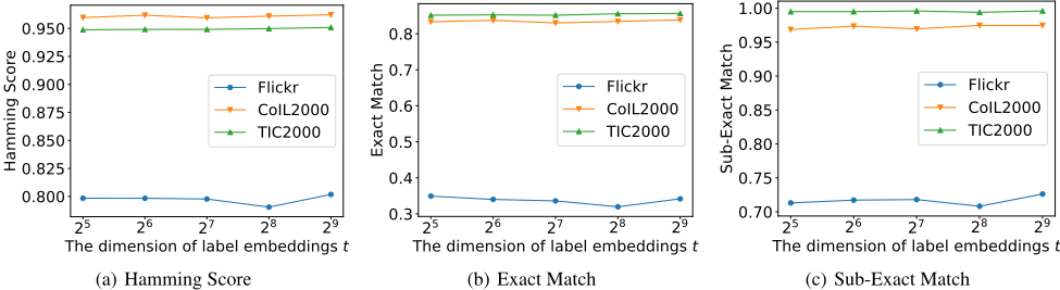
Figure 2 shows how the performance of PIST fluctuates with different values of t, i.e. the dimension of latent label embeddings as mentioned in Eq.(1). It is shown that PIST achieves relatively stable performance when the value of t changed in the range of {25 , 26 , 27 , 28 , 29 }. In this paper, the value of t is set to 25 in light of lower complexity which can be used as the default parameter setting.
5 Conclusion
The main contributions of this paper are two-fold. (1) We propose to consider the specific characteristics contained in different semantic dimensions for MDC which is as important as modeling class dependencies. (2) We proposed a novel MDC approach named PIST which learns pairwise dimension-specific features for MDC to consider both the specific characteristics in each dimension and the dependencies among different dimensions. Experiments clearly validate the effectiveness of the proposed PIST approach.
Acknowledgements
The authors wish to thank the anonymous reviewers for their helpful comments and suggestions. This work was supported by the National Science Foundation of China (62225602, 62306131), and the Big Data Computing Center of Southeast University.
@inproceedings{ijcai2024p462,
  title     = {Deep Multi-Dimensional Classification with Pairwise Dimension-Specific Features},
  author    = {Huang, Teng and Jia, Bin-Bin and Zhang, Min-Ling},
  booktitle = {Proceedings of the Thirty-Third International Joint Conference on
               Artificial Intelligence, {IJCAI-24}},
  publisher = {International Joint Conferences on Artificial Intelligence Organization},
  editor    = {Kate Larson},
  pages     = {4183--4191},
  year      = {2024},
  month     = {8},
  note      = {Main Track},
  doi       = {10.24963/ijcai.2024/462},
  url       = {https://doi.org/10.24963/ijcai.2024/462},
}
TY - CPAPER TI - Deep Multi-Dimensional Classification with Pairwise Dimension-Specific Features AU - Huang, Teng AU - Jia, Bin-Bin AU - Zhang, Min-Ling T2 - Proceedings of the Thirty-Third International Joint Conference on Artificial Intelligence, IJCAI-24 PB - International Joint Conferences on Artificial Intelligence Organization PY - 2024 SP - 4183 EP - 4191 DO - 10.24963/ijcai.2024/462 UR - https://doi.org/10.24963/ijcai.2024/462 ER -Copied
Machine-readable versions of this paper, for tools and AI agents:





