
Negative-Binomial Randomized Gamma Dynamical Systems for Heterogeneous Overdispersed Count Time Sequences
Proceedings of the Thirty-Third International Joint Conference on Artificial Intelligence. Main Track. Pages 4174-4182.
https://doi.org/10.24963/ijcai.2024/461
Keywords
- Uncertainty in AI: UAI: Tractable probabilistic models
- Machine Learning: ML: Bayesian learning
- Machine Learning: ML: Time series and data streams
- Machine Learning: ML: Probabilistic machine learning
Abstract
Modeling count-valued time sequences has been receiving growing interests because count time sequences naturally arise in physical and social domains. Poisson gamma dynamical systems (PGDSs) are newly-developed methods, which can well capture the expressive latent transition structure and bursty dynamics behind count sequences. In particular, PGDSs demonstrate superior performance in terms of data imputation and prediction, compared with canonical linear dynamical system (LDS) based methods. Despite these advantages, PGDS cannot capture the heterogeneous overdispersed behaviours of the underlying dynamic processes. To mitigate this defect, we propose a negative-binomial-randomized gamma Markov process, which not only significantly improves the predictive performance of the proposed dynamical system, but also facilitates the fast convergence of the inference algorithm. Moreover, we develop methods to estimate both factor-structured and graph-structured transition dynamics, which enable us to infer more explainable latent structure, compared with PGDSs. Finally, we demonstrate the explainable latent structure learned by the proposed method, and show its superior performance in imputing missing data and forecasting future observations, compared with the related models.
- [Acharya et al., 2015] Ayan Acharya, Joydeep Ghosh, and Mingyuan Zhou. Nonparametric bayesian factor analysis for dynamic count matrices. In Artificial Intelligence and Statistics, pages 1-9. PMLR, 2015.
- [Acharya et al., 2018] Ayan Acharya, Joydeep Ghosh, and Mingyuan Zhou. A dual markov chain topic model for dynamic environments. In Proceedings of the 24th ACM SIGKDD International Conference on Knowledge Discov- ery & Data Mining, page 1099-1108, 2018.
- [Blei and Lafferty, 2006] David M Blei and John D Lafferty. Dynamic topic models. In Proceedings of the 23rd inter- national conference on Machine learning, pages 113-120, 2006.
- [Chandra et al., 2023] Noirrit Kiran Chandra, Antonio Canale, and David B. Dunson. Escaping the curse of di- mensionality in bayesian model-based clustering. Journal of Machine Learning Research, 24(144):1-42, 2023.
- [Chen et al., 2020] Wenchao Chen, Bo Chen, Yicheng Liu, Qianru Zhao, and Mingyuan Zhou. Switching poisson gamma dynamical systems. In Christian Bessiere, editor, Proceedings of the Twenty-Ninth International Joint Con- ference on Artificial Intelligence, IJCAI-20, pages 2029- 2036. International Joint Conferences on Artificial Intelli- gence Organization, 7 2020. Main track. IJCAI
- [Dieng et al., 2019] Adji B. Dieng, Francisco J. R. Ruiz, and David M. Blei. The dynamic embedded topic model. ArXiv, 2019.
- [Ferguson, 1973] Thomas S. Ferguson. A Bayesian Analysis of Some Nonparametric Problems. The Annals of Statis- tics, 1(2):209 -230, 1973.
- [Filstroff et al., 2021] Louis Filstroff, Olivier Gouvert, Cedric Fevotte, and Olivier Cappe. A comparative study of gamma markov chains for temporal non-negative matrix factorization. IEEE Transactions on Signal Processing, 69:1614 -1626, 2021.
- [Gan et al., 2015] Zhe Gan, Chunyuan Li, Ricardo Henao, David Carlson, and Lawrence Carin. Deep temporal sig- moid belief networks for sequence modeling. In Proceed- ings of the 28th International Conference on Neural In- formation Processing Systems -Volume 2, NIPS'15, page 2467-2475, Cambridge, MA, USA, 2015. MIT Press.
- [Ghahramani and Roweis, 1998] Zoubin Ghahramani and Sam Roweis. Learning nonlinear dynamical systems using an em algorithm. Advances in neural information process- ing systems, 11:431-437, 1998.
- [Han et al., 2014] Shaobo Han, Lin Du, Esther Salazar, and Lawrence Carin. Dynamic rank factor model for text streams. Advances in Neural Information Processing Sys- tems, 27:2663-2671, 2014.
- [Jones et al., 2023] Andrew Jones, F. William Townes, Di- dong Li, and Barbara E. Engelhardt. Alignment of spa- tial genomics data using deep Gaussian processes. Nature Methods, 20(9):1379-1387, 2023.
- [King, 2001] Gary King. Proper nouns and methodological propriety: Pooling dyads in international relations data. In- ternational Organization, 55(2):497-507, 2001.
- [Levitin et al., 2019] Hanna Mendes Levitin, Jinzhou Yuan, Yim Ling Cheng, Francisco JR Ruiz, Erin C Bush, Jef- frey N Bruce, Peter Canoll, Antonio Iavarone, Anna La- sorella, David M Blei, et al. De novo gene signature identi- fication from single-cell rna-seq with hierarchical poisson factorization. Molecular systems biology, 15(2):e8557, 2019.
- [Linderman et al., 2017] Scott Linderman, Matthew John- son, Andrew Miller, Ryan Adams, David Blei, and Liam Paninski. Bayesian Learning and Inference in Recurrent Switching Linear Dynamical Systems. In Proceedings of the 20th International Conference on Artificial Intelli- gence and Statistics, pages 914-922, 2017.
- [Nassar et al., 2018] Josue Nassar, Scott Linderman, Monica Bugallo, and Il Memming Park. Tree-structured recurrent switching linear dynamical systems for multi-scale mod- eling. 2018.
- [Roy and Dunson, 2020] Arkaprava Roy and David B Dun- son. Nonparametric graphical model for counts. The Journal of Machine Learning Research, 21(1):9353-9373, 2020.
- [Rudolph and Blei, 2018] Maja Rudolph and David Blei. Dynamic embeddings for language evolution. In Pro- ceedings of the 2018 World Wide Web Conference, pages 1003--1011, 2018.
- [Schein et al., 2016a] Aaron Schein, Hanna Wallach, and Mingyuan Zhou. Poisson-gamma dynamical systems. Advances in Neural Information Processing Systems, 29:5012-5020, 2016.
- [Schein et al., 2016b] Aaron Schein, Mingyuan Zhou, David Blei, and Hanna Wallach. Bayesian poisson tucker de- composition for learning the structure of international re- lations. In Proceedings of The 33rd International Confer- ence on Machine Learning, pages 2810-2819, 2016.
- [Schein et al., 2019] Aaron Schein, Scott Linderman, Mingyuan Zhou, David Blei, and Hanna Wallach. Poisson-randomized gamma dynamical systems. Ad- vances in Neural Information Processing Systems, 32:782-793, 2019.
- [Sheldon et al., 2013] Daniel Sheldon, Tao Sun, Akshat Ku- mar, and Tom Dietterich. Approximate inference in col- lective graphical models. In Proceedings of the 30th Inter- national Conference on Machine Learning, pages 1004- 1012, 2013.
- [Stewart, 2014] Brandon M Stewart. Latent factor regres- sions for the social sciences. Technical report, Harvard University, 2014.
- [Stuart and Wolfram, 2020] Andrew M. Stuart and Marie- Therese Wolfram. Inverse optimal transport. SIAM Jour- nal on Applied Mathematics, 80(1):599-619, 2020.
- [Tong et al., 2020] Alexander Tong, Jessie Huang, Guy Wolf, David Van Dijk, and Smita Krishnaswamy. Trajec- torynet: A dynamic optimal transport network for model- ing cellular dynamics. In Proceedings of the 37th Interna- tional Conference on Machine Learning, 2020.
- [Virtanen and Girolami, 2020] Seppo Virtanen and Mark Girolami. Dynamic content based ranking. In Proceedings of the Twenty Third International Conference on Artificial Intelligence and Statistics, pages 2315-2324, 2020.
- [Wang et al., 2008] Chong Wang, David M. Blei, and David E. Heckerman. Continuous time dynamic topic models. In Conference on Uncertainty in Artificial Intelli- gence, 2008.
- [Zhou and Carin, 2012] Mingyuan Zhou and Lawrence Carin. Augment-and-conquer negative binomial pro- cesses. In Advances in Neural Information Processing Systems, volume 25, pages 2546-2554.
- Curran Associates, Inc., 2012.
- [Zhou and Carin, 2015] Mingyuan Zhou and Lawrence Carin. Negative binomial process count and mixture modeling. IEEE Trans. Pattern Anal. Mach. Intell., 37(2):307-320, 2015.
- [Zhou et al., 2016] Mingyuan Zhou, Yulai Cong, and Bo Chen. Augmentable gamma belief networks. Journal of Machine Learning Research, 17(163):1-44, 2016.
- [Zhou, 2015] Mingyuan Zhou. Infinite Edge Partition Mod- els for Overlapping Community Detection and Link Pre- diction. In Proceedings of the Eighteenth International Conference on Artificial Intelligence and Statistics, pages 1135-1143, 2015.
- [Zhou, 2016a] Mingyuan Zhou. Nonparametric bayesian negative binomial factor analysis. Bayesian Analysis, 13(4):1065-1093, 2016.
- [Zhou, 2016b] Mingyuan Zhou. Softplus regressions and convex polytopes, 2016.
- [Zhou, 2018] Mingyuan Zhou. Parsimonious bayesian deep networks. In Advances in Neural Information Processing Systems, 2018.
References were extracted automatically from the PDF and may contain errors.
Full text extracted automatically from the PDF; figures, tables and equations may differ. The PDF is the version of record.
1 Introduction
Count time sequences, naturally arise in many domains such as text mining [Blei and Lafferty, 2006; Wang et al., 2008; Rudolph and Blei, 2018; Acharya et al., 2018; Dieng et al., 2019], cell genomic analysis [Levitin et al., 2019; Tong et al., 2020; Jones et al., 2023], population movement forecasting [Sheldon et al., 2013; Stuart and Wolfram, 2020; Roy and Dunson, 2020], and etc. Modeling count sequences has been drawing increasing research attention because these real-world count data usually exhibit bursty and overdispersed behaviours, which cannot be well-captured by canonical linear dynamical systems (LDSs) [Ghahramani and Roweis, 1998]. In addition, some previous works use extended rank likelihood functions [Han et al., 2014] which link the count observations to latent continuous dynamics to model count time sequences. Nonetheless, the extended rank likelihood functions cannot faithfully capture bursty dynamics underlying real-world count sequences. Meanwhile, the extended rank likelihood functions often require an approximate inference scheme, and thus scale poorly with highdimensional count sequences, such as single-cell RNA sequencing data [Chandra et al., 2023]. Notably, some recent works [Acharya et al., 2015; Schein et al., 2016a; Schein et al., 2016b; Schein et al., 2019] model sequential count observations using gamma Poisson family distributions. More specifically, [Acharya et al., 2015] develops a gamma Markov process to capture continuous dynamics underlying count-valued sequences. In particular, the number of latent factors behind high-dimensional count data, can be appropriately determined by the gamma process prior, in a Bayesian non-parametric manner. Following the success of [Acharya et al., 2015], Schein et al. [2016a] study a Poisson gamma dynamical system, in which a transition kernel is designed to capture how the latent dimensions interact with each other to model complicated observed dynamics. Another appealing aspect of the Poisson gamma dynamic model is that the posterior simulation can be performed using a tractable-yet-efficient Gibbs sampling algorithm via Poisson-Logarithm data augmentation strategy [Zhou and Carin, 2012; Zhou and Carin, 2015]. Hence, the Poisson gamma dynamic models [Acharya et al., 2015; Schein et al., 2016a; Schein et al., 2019] are in particular well-fitted to impute missing entries, to predict future unseen observations and to estimate uncertainties.
∗Corresponding Author.
Despite these advantages, these models still cannot well capture the heterogeneous overdispersion effects of the latent dynamic processes behind count observations. For instance, international event data, usually consists of multiple latent dynamic processes, which often change rapidly with the different magnitudes [King, 2001; Stewart, 2014]. To capture such heterogeneous overdispersed behaviours, we develop a negative-binomial-randomized gamma Markov chain structure, which not only greatly enhances the model flexibility, but also facilitates the fast convergence of the derived Gibbs sampling algorithms. Moreover, the transition dynamics behind real-world high-dimensional count data, are often sparse, and exhibit a certain amount of graph structure. Hence, we propose to learn the graph-structured transition dynamics using relational gamma processes [Zhou, 2015]. To the best of our knowledge, this is the first attempt to learn the latent graph-structured transition dynamics under the Poisson gamma dynamical system.
The main contributions of the paper include: 1) A negativebinomial-randomized gamma Markov process (NBRGMP) is proposed to estimate the heterogeneous overdispersion effects of the latent dimensions underlying sequential count observations; 2) Relational gamma processes are thoroughly studied to learn both factor-structured and graph-structured transition dynamics, which renders the estimated latent structure more explainable, compared with transition structure inferred using non-informative priors; 3) Although the proposed NBRGMP and its factor-structured and graphstructured extensions are intractable, simple-yet-efficient Gibbs sampling algorithms are developed via Negativebinomial data augmentation strategies to perform inference; 4) Extensive experiments are conducted to illustrate the explainable transition structure learned by the proposed model. We demonstrate the superior performance of the proposed method in missing data imputation and future snapshot forecasting, with several related works.
2 Preliminary
Suppose we have a sequentially-observed count data over time interval [0, T ] specified by N = (n1, . . . , nV )T of V dimensions, where nv = (n(1) v , . . . , n(T) v )T with n(t) v denoting the v-th observation at time t. The Poisson gamma dynamical system [Schein et al., 2016a] models the count n(t) v as
where θ(t) k captures the strength of latent component k at time t, and ϕvk represents the involvement degree of dimension v in latent component k. To model the underlying dynamics, the PGDS assumes that the latent components evolve over time according to a gamma Markov chain structure as
where the latent components θ(t-1) = (θ(t-1) 1 , . . . , θ(t-1) K )T evolve over time through the transition matrix Π. The θ(t-1) k captures how strongly the k-th latent component activates at time t-1, and πkk2 models how strongly the k2-th component θ(t-1) k2 at time t - 1 affect the k-th component θ(t) k at time t. Eq. 2 naturally defines a gamma Markov chain structure. The expectation and variance of the gamma Markov chain can be calculated respectively as E[θ(t) | θ(t-1) ,Π] =Πθ(t-1) and Var[θ(t) | θ(t) ,Π] = (Πθ(t-1) )τ -1 0 , where τ0 controls the variance of θ(t) .
Schein et al. [2019] further develop a Poisson-randomized gamma Markov chain (PRGMC) structure specified by
By marginalizing out the Poisson latent states h(t) k , we have a continuous-valued dynamical system given by
where RG1 is the randomized gamma distribution of the first type. The marginal expectation and variance of the PRGMC is E[θ(t) | θ(t-1) ,Π] = Πθ(t-1) + ϵ(θ) 0 τ -1 and Var[θ(t) | θ(t-1) ,Π] = 2Πθ(t-1) τ -1 + ϵ(θ) 0 τ -2 , respectively.
3 The ProposedModel
In this section we will introduce the novel negative-binomialrandomized gamma Markov chain structure to capture the heterogeneous overdispersion effects of the latent dimensions behind count data. Then we shall describe how to learn explainable latent transition structure with relational gamma processes. The proposed negative-binomialrandomized gamma dynamical system is defined by
where δ(t) is a nonnegative multiplicative term capturing time-dependent bursty dynamics. We place a gamma prior on δ(t) as δ(t) ∼ Gam(ϵ0, ϵ0), and let δ(t) = δ if the generative process (Eq. 3) is stationary over time. Here ϕk = (ϕ1k, ϕ2k, . . . , ϕV k)T denotes the loading coefficient of k-th latent component, and λk denotes the weight of k-th latent component. To ensure model identifiability, we require ∑v ϕvk = 1 and thus have a Dirichlet prior over ϕk given by ϕk ∼ Dir(ϵ0, ..., ϵ0). More specifically, we draw λk from a hierarchical prior as λk ∼ Gam( ϵ(λ) 0K + gk, β), in which gk ∼ Pois( γK ). We specify gamma priors over γ and β as γ ∼ Gam(ϵ0, ϵ0), β ∼ Gam(ϵ0, ϵ0). Note that as K → ∞, the summation of the weight expectation remains finite and fixed, i.e., ∑∞k=1 E[λk] = β-1 (ϵ(λ) 0 + γ). Hence, this hierarchical prior enables us to effectively estimate a finite number of latent factors that are representative to capture the temporal dynamics.
3.1 Negative-Binomial Randomized Gamma Markov Processes
To capture the heterogeneous overdispersed behaviors of the latent dimensions behind count sequences, we introduce a negative-binomial randomized gamma Markov process (NBRGMP) specified by
where we set θ(0) k = λk, and θ(t) k is gamma distributed with shape parameter ϵ(θ) 0 + h(t) k where ϵ(θ) 0 ≥ 0, and the rate parameter τ. Here, instead of specifying a Poisson prior as did in [Schein et al., 2019], we draw the intermediate latent state h(t) k from a negative-binomial distribution to enhance the flexibility of θ(t) k , which enable us to estimate the heterogeneous overdispersed behaviours of the latent dynamic processes. More specifically, the marginal expectation and variance of the NBRGMP can be calculated by iteration as
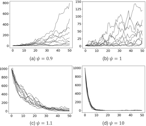
respectively. We note that both the concentration parameter τ and hyperparameter ϵ(θ) 0 appear in the additive term of the expectation and variance, which can be concealed by letting ϵ(θ) 0 = 0. The hyperparameter ψ plays a crucial role in controlling the variance of the NBRGMP. More specifically, when ψ ∈ (0, 1) the values of θ(t) will fluctuate dramatically because of its large expectation and variance. When ψ = 1, the expectation of the NBRGMP will be the same with the PRGMC (as discussed in Sec. 2), while the variance of the NBRGMP will be three times of the variance of the PRGMC, which thus allows the proposed dynamical system to capture reasonable heterogeneous overdispersed behaviors. When ψ ∈ (1, 1 + √2), the expectation of the NBRGMP will tend to be smaller compared with the expectation of the PRGMC, which will be more suitable to capture sparse counts. Meanwhile, the variance of the NBRGMP still allows us to capture a limited range of overdispersion effects. If ψ ≥ 1+ √2, both expectation and variance converge to zeros as ψ goes to infinity. Fig. 1 plots the realizations of the NBRGMP by varying the parameter ψ. Note that the negative-binomial distributed latent state h(t) k can be equivalently drawn from a gammaPoisson mixture as
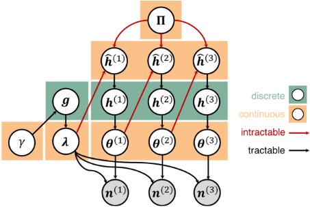
Fig. 2 shows the graphical representation of the developed NBRGMP. When τ ∑k2 πkk2 θ(t-1) k2 → ∞, the h(t) k is approximately characterized by Pois( τψ ∑k2 πkk2 θ(t-1) k2 ). Hence, by marginalizing the Poisson distributed latent states h(t) k from Eq. 4, the negative-binomial randomized gamma dynamical system can be equivalently represented by randomized gamma distribution of the first type as
3.2 Factor-structured Transition Dynamics
We first propose to learn the latent factor structure behind transition dynamics. To that end, we specify a hierarchical Dirichlet prior over πk as πk ∼ Dir(a1k, . . . , aKk),where ak = (a1k, . . . , aKk)T is the hyper-parameter. Our goal here is to capture the correlation structure between the latent dimensions of the transition kernel. Thus, we model the hyperparameter A = [ak1k2 ]Kk1,k2 using a Poisson factor model as
where rc is the weight of c-th latent factor, and mkc captures how strongly k-th component associates with c-th factor. Naturally, k1-th component interact with k2-th component through the weight ∑Cc=1 mk1crcmk2c. To ensure the latent factor to be nonnegative, we draw the factor rc, and factor loading mkc from the priors specified by
respectively. Here, C is the maximum number of latent factors. As C → ∞, the weights of the latent factors {rc}Cc and the factor loading {mc}Cc can be considered as a draw G = ∑∞c=1 rcδmc from a gamma process GaP(G0, c0), where G0 denotes the base measure over the metric space Ω, and c0 the concentration parameter [Ferguson, 1973].
3.3 Graph-Structured Transition Dynamics
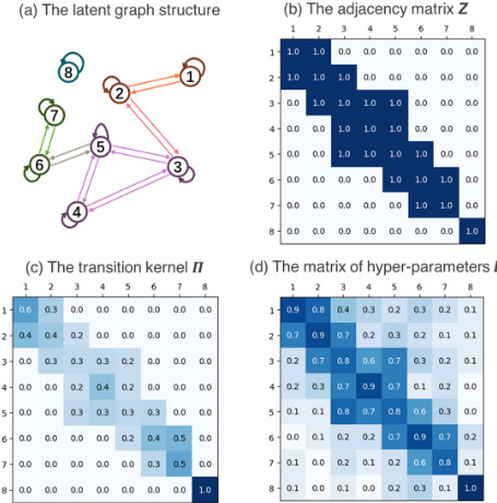
For high-dimensional count sequences, the underlying transition dynamics are often sparse and exhibit a certain amount of graph structure. Hence, we further study to learn the latent graph-structured transition kernel behind count time series, using relational gamma process prior. In particular, we sample the transition parameter πk from a hierarchical Dirichlet prior, as πk ∼ Dir(a1k, . . . , aKk). To introduce a sparse graph-structured transition kernel, we model the matrix of the hyper-parameter A = [ak1k2 ]Kk1,k2 as A = D ⊙ Z, where D = [dk1k2 ]Kk1,k2 denotes the matrix of the nonnegative hyper-parameters, and Z = [zk1k2 ]Kk1,k2 is a binary mask. More specifically, we consider the dimensions of the transition kernel as vertices, and the non-zero transition behaviours as graph edges. Naturally, we can capture the sparse structure of the transition kernel Π using a graph. As shown in Fig. 3, for each pair of two vertices i and j, zij = 1 means that the transition probability from i-th component to j-th component is non-zero, and vice versa. In particular, we model the binary mask Z using relational gamma processes as
where rc can be considered as the weight of latent community c, and mkc measures how strongly k-th vertex (the dimension of the transition kernel) relate to c-th latent community, as illustrated in Fig. 3. Note that the binary mask Z can be equivalently drawn via the Bernoulli-Poisson link function as
To ensure the model explainability, we restrict rc and mkc to be nonnegative, and thus place gamma priors over these two parameters as mkc ∼ Gam(ˆak, ˆbk), rc ∼ Gam( r0 C , c0), respectively. As we discussed in Sec. 3.2, this hierarchical gamma prior can be considered as a draw G = ∑∞c=1 rcδmc from a gamma process GaP(G0, c0). In particular, we call this Bayesian non-parametric prior the relational gamma process, as a graph-structure can be naturally induced. The nonnegative hyper-parameters D = [dk1k2 ]Kk1,k2 are drawn from a gamma distribution as dk1k2 ∼ Gam(ϵ0, ϵ0).
The proposed gamma dynamical systems are not fully conjugate. Nonetheless, tractable-yet-efficient Gibbs sampling algorithms are developed to perform posterior simulation via negative-binomial data augmentation strategies [Zhou, 2016a]. The full derivation of the inference procedure is presented in the supplementary material.
4 RelatedWork
Modeling sequentially observed count sequences has been receiving growing interests in recent years. Here we discuss several types of methods closely related to our studies. [Acharya et al., 2015] first studies the gamma Markov process on sequentially count sequences, in which the latent states evolve independently over time. [Schein et al., 2016a] tries to capture the excitations among the latent gamma Markov processes using a transition structure. [Schein et al., 2019] investigates a Poisson-randomized gamma Markov process which can capture a certain amount of bursty dynamics, and thus demonstrates advantages over gamma Markov processes. [Virtanen and Girolami, 2020] studies a second type of gamma Markov chain structure via the scale parameter of the latent gamma states, which demonstrate better stationary property over the gamma Markov chain proposed by [Acharya et al., 2015]. [Filstroff et al., 2021] recently provides a thorough survey on the studies of the developed gamma Markov processes, and evaluates these models through standard tasks including data smoothing and forecasting. [Han et al., 2014] first tries to capture sequential count observations using linear dynamical systems, via the extend rank likelihood function. [Linderman et al., 2017] proposes to learn switching behaviors of sequential data using recurrent linear dynamical systems (rLDS). [Nassar et al., 2018] further develops a tree-structured extension of rLDS, with multi scale resolution. [Chen et al., 2020] extends the Poisson gamma dynamical systems to learn non-stationary transition dynamics behind count time series. Some efforts are also dedicated to developing Bayesian deep models to capture count sequences. [Gan et al., 2015] develops a temporal sigmoid belief network for count time series.
5 Experiments
We evaluate the proposed relational gamma process dynamical systems, and compare it with closely-related methods, using both synthetic and real-world count data.
Real-world data. We conducted the experiments with the following real-world datasets: (1) Integrated Crisis Early Warning System (ICEWS) dataset contains the count number of 6, 000 pairwise interactions between 233 countries over 365 days. By screening out 4, 800 dimensions where the sample sparsity exceeds 99%, we used a subset of ICEW data which contains V = 1, 200 dimensions, and T = 365 time steps; (2) Last.fm contains the listening information of 7, 071 music artists over 51 months, where we have T = 51 time steps, and V = 7, 071 dimensions; (3) Earthquake Reports Database (EQDB): records more than 120, 000 earthquake reports over 15, 000 earthquakes whose epicenters in the United States and nearby U.S. territories from 1928 to 1985. We created a count matrix where each column represents a month and each row represents a state. The EQDB used in the experiments, contains T = 696 time steps, and V = 64 dimensions. (4) COVID-19 contains the daily death toll in the fifty states and Washington DC of the United States, from March 2020 to March 2021. We have T = 365 time steps, and V = 51 dimensions.
Baselines. In the experiments we compared the predictive of the proposed models with (1) the gamma process dynamic Poisson factor analysis (GaP-DPFA) [Acharya et al., 2015], in which the gamma Markov chain evolves independently over time; (2) the Poisson-gamma dynamical system (PGDS) [Schein et al., 2016a], in which a transition kernel is used to capture the excitations among latent gamma Markov chains; (3) the Poisson-randomized gamma dynamical system (PRGDS) [Schein et al., 2019] where the Poissonrandomized gamma Markov chain structure can capture a certain amount of bursty dynamics.
We denote the proposed negative-binomial-randomized gamma dynamical system as NBRGDS. The proposed NBRGDS with factor-structured prior imposed over the transition kernel, is denoted as FS-NBRGDS. The proposed NBRGDS with graph-structured prior placed over the transition structure, is denoted by GS-NBRGDS.
To evaluate the performance of the compared models in capturing heterogeneous overdispersed behaviours of latent dynamic processes behind count sequences, we considered a subset of ICEWS data that consists of heterogeneous overdispersed counts. More specifically, we sorted the oberserved dimensions according to their variance/expectation ratio, and selected the first L dimensions in descending order, i.e., those dimensions with larger variation/expectation ratio. We present the result for the setting L = 300. We treated the 80 percent of the data as the training set, and the remaining 20 percent as the test set. Then, we trained all the compared models with the training set, and evaluated the model performance using the test set. In the experiments, we used mean absolute error (MAE) and mean relative error (MRE) to evaluate the model performance in fitting count sequences:
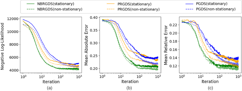
where n(t) v and ˆn(t) v denotes the ground true value and estimated value of dimension v at time t, respectively. They differ because MRE considers the relative magnitude of the errors in relation to the actual values, taking into account the scale of the data, while MAE simply measures the absolute magnitude of the errors without considering the data scale. Fig. 4 shows the results of the compared models averaged over ten random training-testing repeats.
As shown in Fig. 4 (a), NBRGDS has started to converge to its steady states after almost 102 iterations, while both PGDS and PRGDS start to converge until 103 iterations. Fig. 4 (b) and (c) compares the mean absolute errors and mean relative errors of the compared models, respectively. Overall, NBRGDS achieves the lowest MAE and MRE. PRGDS performs better than PGDS as PRGDS can capture a certain amount of overdispersion effects via its Poisson-randomized chain structure. We also note that NBRGDS with a timevaring scaling factor δ(t) , performs better than stationary NBRGDS because this scaling factor δ(t) can also capture bursty dynamics. Nonetheless, stationary NBRGDS still outperforms both the PRGDS and PGDS with time-varing δ(t) . We conjecture that this improved prediction accuracy is because the time-varying scaling factor δ(t) fail to capture the underlying overdispersed behaviours, although it still can model a certain amount of bursty dynamics in observed dimensions. This observation further demonstrates the strong ability of the NBRGDS in capturing hetergeneous overdispersion effects of the latent dimensions behind count sequences.
| GaP-DPFA | PGDS | PRGDS | NBRGDS | FS-NBRGDS | GS-NBRGPDS | ||
|---|---|---|---|---|---|---|---|
| ICEWS | MAE | S 1.29±0.01 | 1.04±0.02 | 1.06±0.01 | 1.04±0.00 | 1.04±0.01 | 1.04±0.01 |
| F 0.94±0.01 | 0.95±0.03 | 0.98±0.04 | 1.12±0.02 | 0.91±0.02 | 0.90±0.01 | ||
| MRE | S 0.61±0.00 | 0.41±0.01 | 0.42±0.00 | 0.43±0.01 | 0.42±0.00 | 0.41±0.02 | |
| F 0.53±0.01 | 0.51±0.04 | 0.59±0.03 | 0.58±0.02 | 0.54±0.01 | 0.51±0.01 | ||
| Last.fm | MAE | S 1.71±0.03 | 1.38±0.01 | 1.39±0.01 | 1.37±0.01 | 1.36±0.02 | 1.38±0.02 |
| F 8.04±0.07 | 1.41±0.02 | 5.47±0.22 | 1.41±0.02 | 1.12±0.01 | 1.13±0.02 | ||
| MRE | S 0.52±0.01 | 0.34±0.01 | 0.34±0.00 | 0.34±0.01 | 0.33±0.00 | 0.34±0.00 | |
| F 4.02±0.04 | 0.86±0.02 | 2.59±0.09 | 0.85±0.03 | 0.53±0.04 | 0.53±0.01 | ||
| EQDB | MAE | S 3.37±0.09 | 3.37±0.20 | 3.41±0.33 | 3.26±0.12 | 3.26±0.20 | 3.34±0.27 |
| F 10.17±2.21 | 10.89±0.94 | 7.08±0.90 | 5.65±0.63 | 3.55±0.04 | 3.33±0.06 | ||
| MRE | S 0.89±0.17 | 0.89±0.05 | 0.84±0.08 | 0.83±0.09 | 0.83±0.07 | 0.82±0.05 | |
| F 8.12±2.14 | 6.54±0.93 | 2.45±0.46 | 1.49±0.11 | 1.52±0.15 | 1.40±0.10 | ||
| COVID-19 | MAE | S 12.09±0.26 | 11.42±0.62 | 11.08±0.25 | 10.99±0.43 | 11.57±0.07 | 11.37±0.62 |
| F 23.35±1.07 | 27.67±0.18 | 21.95±0.59 | 20.87±0.29 | 23.55±0.08 | 23.30±0.05 | ||
| MRE | S 1.47±0.19 | 1.54±0.11 | 1.23±0.11 | 1.19±0.13 | 1.41±0.22 | 1.32±0.11 | |
| F 6.30±0.58 | 7.87±0.32 | 6.32±0.32 | 1.94±0.15 | 1.36±0.03 | 1.40±0.03 |
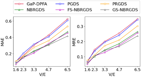
Synthetic data. To further evaluate the performance of the compared models in capturing overdispersion effects, we also considered generating synthetic data with heterogeneous overdispersed dynamics. To that end, we considered to simulate synthetic data using zero-inflated negative-binomial (ZINB) models given by
where fZINB and fNB represents the probability mass function (PMF) of the zero-inflated negative-binomial distribution and negative-binomial distribution, respectively. Here, I0(n) is an indicator function that takes 1 when n = 0, otherwise
0. The parameter p0 ∈ [0, 1] controls the ratio of zero counts, while r and p are the two parameters of the negative-binomial distribution. Hence, we can effectively control the sparsity and overdispersion magnitude of the dimensions by tuning the values of p0 and p, respectively 1 . More specifically, we generated five groups of synthetic data, in which each group contains V = 10 dimensions and T = 365 time steps, using the following configurations: (1) p0 = 0.9, r = 5, p = 0.9, V/E = 1.6; (2) p0 = 0.9, r = 5, p = 0.8, V/E = 2.3; (3) p0 = 0.9, r = 5, p = 0.7, V/E = 3.3; (4) p0 = 0.9, r = 5, p = 0.6, V/E = 4.7; (5) p0 = 0.9, r = 5, p = 0.5, V/E = 6.5, where V and E represents variance and expectation of each group data, respectively. Then V/E denotes the ratio of variance to expectation, and thus measures overdispersion effects. Fig. 5 plots the model performance of the compared methods by varying the ratio of variance to expectation. NBRGDS models including its factor-structured and graph-structured versions, consistently outperforms the other methods. In particular, NBRGDS achieves a significant improvement compared with PRGDS, although PRGDS still can capture a certain amount of overdispersion effects. Additional experiments on synthetic data under different configurations are available in the supplementary material.
Data Smoothing and Forecasting. To quantatively evaluate the predictive performance of the compared methods, we considered two standard tasks: data smoothing and future data forecasting. The data smoothing is to predict y(t) v given the remaining observations y(1:T) v \ y(t) v , while the future data prediction is to predict future observations at next S time steps y(T+1):(T+S) v given the history up to T, y(1:T) v . Here we considered to predict next two time steps (S = 2). We used the default settings of GaP-DPFA, and PRGDS as provided in the corresponding releases [Acharya et al., 2015; Schein et al., 2019]. For NBRGDS, FS-NBRGDS and GSNBRGDS, we choose K = 100 when V ≥ 1000, while the dimensions of EQDB and COVID-19 datasets are smaller than 100, thus we choos K = 25. We set C = K for FSNBRGDS and GS-NBRGDS. We ran 5000 iterations of the Gibbs sampler, which have started to converge after 1000 iterations. We discarded the first 3000 samples which were treated as burn-in time and collected a posterior sample every tenth sample thereafter. Tab. 1 shows the results of the compared methods in these two tasks. Overall, NBRGDS outperforms the GaP-DPFA, PGDS and PRGDS on almost all the datasets. In particular, we found that FS-NBRGDS and GS-NBRGDS show superior performance in future data forecasting. We conjecture this improved prediction accuracy is due to that FS-NBRGDS and GS-NBRGDS can effectively leverage the structure information underlying dynamic count data, and thus yields better predictive accuracy. We provide more comparative results on data smoothing and forecasting over different models in appendix Sec.D.
1 Assume an random variable x ∼ ZINB(p0, r, p). The expectation and variance of x are E[x] = r(1 - p0)(1 - p)/p, and Var[x] = (1 - p0)r(1 - p)/p2 + p0(1 - p0)r2 (1 - p)2 /p2 , respectively. Thus, the ratio of variance to expectation of x is (1 + rp0(1 - p))/p.
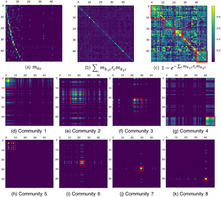
Graph-Structured Transition Dynamics. Fig. 6 shows the latent graph structure underlying the transition kernel, estimated by the proposed model. Although the model was initialized with C = 50 latent communities, the latent graph only consists of approximately ten communities with nonzero weights, as shown in Fig. 6(a). Fig. 6(d-k) plots the eight evident latent communities in which the vertices are densely connected as the corresponding dimensions are more likely to interact with each other. Fig. 6(c) demonstrates that the most estimated latent dynamic processes are almost independent to the other dynamic processes, but only interact with a few other dimensions. We provide the latent graphs inferred for the other real-world data in the supplement.
6 Conclusion
Novel negative-binomial-randomized gamma dynamical systems, have been proposed to capture the heterogeneous overdispersed behaviors of latent dynamics behind count time sequences. The new framework demonstrates more explainable latent structure, by learning the factor structure and sparse graph structure of the transition kernels, compared with transition kernel by non-informative priors. Although the prior specification of the proposed framework lacks conjugacy, tractable-yet-efficient sampling algorithms are developed to perform posterior inference. In the future, we plan to capture time-varying graph-structured transition dynamics, which will enable to better understand non-stationary count sequences. We are also considering to enhance the modeling capacities of gamma belief networks [Zhou et al., 2016; Zhou, 2018] and convex polytopes [Zhou, 2016b] using the negative-binomial-randomized gamma Markov processes.
Acknowledgments
This work was partly supported by the Guangdong Provincial Key Laboratory of Mathematical and Neural Dynamical Systems.
@inproceedings{ijcai2024p461,
  title     = {Negative-Binomial Randomized Gamma Dynamical Systems for Heterogeneous Overdispersed Count Time Sequences},
  author    = {Huang, Rui and Yang, Sikun and Koeppl, Heinz},
  booktitle = {Proceedings of the Thirty-Third International Joint Conference on
               Artificial Intelligence, {IJCAI-24}},
  publisher = {International Joint Conferences on Artificial Intelligence Organization},
  editor    = {Kate Larson},
  pages     = {4174--4182},
  year      = {2024},
  month     = {8},
  note      = {Main Track},
  doi       = {10.24963/ijcai.2024/461},
  url       = {https://doi.org/10.24963/ijcai.2024/461},
}
TY - CPAPER TI - Negative-Binomial Randomized Gamma Dynamical Systems for Heterogeneous Overdispersed Count Time Sequences AU - Huang, Rui AU - Yang, Sikun AU - Koeppl, Heinz T2 - Proceedings of the Thirty-Third International Joint Conference on Artificial Intelligence, IJCAI-24 PB - International Joint Conferences on Artificial Intelligence Organization PY - 2024 SP - 4174 EP - 4182 DO - 10.24963/ijcai.2024/461 UR - https://doi.org/10.24963/ijcai.2024/461 ER -Copied
Machine-readable versions of this paper, for tools and AI agents:





