
Perturbation Guiding Contrastive Representation Learning for Time Series Anomaly Detection
Proceedings of the Thirty-Third International Joint Conference on Artificial Intelligence. Main Track. Pages 4955-4963.
https://doi.org/10.24963/ijcai.2024/548
Keywords
- Machine Learning: ML: Representation learning
- Machine Learning: ML: Time series and data streams
- Machine Learning: ML: Unsupervised learning
- Machine Learning: ML: Self-supervised Learning
Abstract
Time series anomaly detection is a critical task with applications in various domains. Due to annotation challenges, self-supervised methods have become the mainstream approach
for time series anomaly detection in recent years. However,
current contrastive methods categorize data perturbations into
binary classes, normal or anomaly, which lack clarity on the specific impact of different perturbation methods. Inspired by the hypothesis that "the higher the probability of misclassifying perturbation types, the higher the probability of anomalies", we propose PCRTA, our
approach firstly devises a perturbation classifier to learn the
pseudo-labels of data perturbations. Furthermore, for addressing "class collapse issue" in contrastive learning, we propose a perturbation guiding positive and negative samples
selection strategy by introducing learnable perturbation classification networks. Extensive experiments on six realworld datasets demonstrate the significant superiority of our
model over thirteen state-of-the-art competitors, and obtains average
5.14%, 8.24% improvement in F1 score and AUC-PR, respectively.
- [Aggarwal and Aggarwal, 2017] Charu C Aggarwal and Charu C Aggarwal. An introduction to outlier analysis. Springer, 2017.
- [Ahmed et al., 2023] Sabeen Ahmed, Ian E Nielsen, Aakash Tripathi, Shamoon Siddiqui, Ravi P Ramachandran, and Ghulam Rasool. Transformers in time-series analysis: A tutorial. Circuits, Systems, and Signal Processing, 42(12):7433-7466, 2023.
- [Audibert et al., 2020] Julien Audibert, Pietro Michiardi, Frédéric Guyard, Sébastien Marti, and Maria A Zuluaga. Usad: Unsupervised anomaly detection on multivariate time series. In Proceedings of the 26th ACM SIGKDD international conference on knowledge discovery & data mining, pages 3395-3404, 2020.
- [Bai et al., 2018] Shaojie Bai, J Zico Kolter, and Vladlen Koltun. An empirical evaluation of generic convolutional and recurrent networks for sequence modeling. arXiv preprint arXiv:1803.01271, 2018.
- [Baireddy et al., 2021] Sriram Baireddy, Sundip R Desai, James L Mathieson, Richard H Foster, Moses W Chan, Mary L Comer, and Edward J Delp. Spacecraft time-series anomaly detection using transfer learning. In Proceedings of the IEEE/CVF Conference on Computer Vision and Pat- tern Recognition, pages 1951-1960, 2021.
- [Bergman and Hoshen, 2020] Liron Bergman and Yedid Hoshen. Classification-based anomaly detection for gen- eral data. In 8th International Conference on Learning Representations, ICLR 2020, Addis Ababa, Ethiopia, April 26-30, 2020, 2020.
- [Breunig et al., 2000] Markus M Breunig, Hans-Peter Kriegel, Raymond T Ng, and Jörg Sander. Lof: iden- tifying density-based local outliers. In Proceedings of the 2000 ACM SIGMOD international conference on Management of data, pages 93-104, 2000.
- [Campos et al., 2021] David Campos, Tung Kieu, Chenjuan Guo, Feiteng Huang, Kai Zheng, Bin Yang, and Chris- tian S Jensen. Unsupervised time series outlier detection with diversity-driven convolutional ensembles-extended version. arXiv preprint arXiv:2111.11108, 2021.
- [Chandola et al., 2009] Varun Chandola, Arindam Banerjee, and Vipin Kumar. Anomaly detection: A survey. ACM computing surveys (CSUR), 41(3):1-58, 2009.
- [Chen et al., 2020] Ting Chen, Simon Kornblith, Moham- mad Norouzi, and Geoffrey Hinton. A simple framework for contrastive learning of visual representations. In In- ternational conference on machine learning, pages 1597- 1607. PMLR, 2020.
- [Chuang et al., 2020] Ching-Yao Chuang, Joshua Robinson, Yen-Chen Lin, Antonio Torralba, and Stefanie Jegelka. Debiased contrastive learning. Advances in neural infor- mation processing systems, 33:8765-8775, 2020.
- [Deng and Hooi, 2021] Ailin Deng and Bryan Hooi. Graph neural network-based anomaly detection in multivariate time series. In Proceedings of the AAAI conference on artificial intelligence, volume 35, pages 4027-4035, 2021.
- [Eldele et al., 2021] Emadeldeen Eldele, Mohamed Ragab, Zhenghua Chen, Min Wu, Chee Keong Kwoh, Xiaoli Li, and Cuntai Guan. Time-series representation learning via temporal and contextual contrasting. In Proceedings of the Thirtieth International Joint Conference on Artificial Intelligence, IJCAI-21, pages 2352-2359, 8 2021. IJCAI
- [Garg et al., 2021] Astha Garg, Wenyu Zhang, Jules Sama- ran, Ramasamy Savitha, and Chuan-Sheng Foo. An eval- uation of anomaly detection and diagnosis in multivariate time series. IEEE Transactions on Neural Networks and Learning Systems, 33(6):2508-2517, 2021.
- [Golan and El-Yaniv, 2018] Izhak Golan and Ran El-Yaniv. Deep anomaly detection using geometric transformations. Advances in neural information processing systems, 31, 2018.
- [Gupta et al., 2013] Manish Gupta, Jing Gao, Charu C Ag- garwal, and Jiawei Han. Outlier detection for temporal data: A survey. IEEE Transactions on Knowledge and data Engineering, 26(9):2250-2267, 2013.
- [Hadsell et al., 2006] Raia Hadsell, Sumit Chopra, and Yann LeCun. Dimensionality reduction by learning an invariant mapping. In 2006 IEEE computer society conference on computer vision and pattern recognition (CVPR'06), vol- ume 2, pages 1735-1742. IEEE, 2006.
- [Hautamaki et al., 2004] Ville Hautamaki, Ismo Karkkainen, and Pasi Franti. Outlier detection using k-nearest neigh- bour graph. In Proceedings of the 17th International Con- ference on Pattern Recognition, 2004. ICPR 2004., vol- ume 3, pages 430-433. IEEE, 2004.
- [He et al., 2020] Kaiming He, Haoqi Fan, Yuxin Wu, Sain- ing Xie, and Ross Girshick. Momentum contrast for unsu- pervised visual representation learning. In Proceedings of the IEEE/CVF conference on computer vision and pattern recognition, pages 9729-9738, 2020.
- [Hyvarinen and Morioka, 2016] Aapo Hyvarinen and Hi- roshi Morioka. Unsupervised feature extraction by time- contrastive learning and nonlinear ica. Advances in neural information processing systems, 29, 2016.
- [Jiehui Xu and Long, 2022] Jianmin Wang Jiehui Xu, Haixu Wu and Mingsheng Long. Anomaly transformer: Time series anomaly detection with association discrep- ancy. In The Tenth International Conference on Learning Representations, ICLR 2022, Virtual Event, April 25-29, 2022, 2022.
- [Lai et al., 2021] Kwei-Herng Lai, Daochen Zha, Junjie Xu, Yue Zhao, Guanchu Wang, and Xia Hu. Revisiting time series outlier detection: Definitions and benchmarks. In Thirty-fifth conference on neural information processing systems datasets and benchmarks track (round 1), 2021.
- [Li et al., 2019] Dan Li, Dacheng Chen, Baihong Jin, Lei Shi, Jonathan Goh, and See-Kiong Ng. Mad-gan: Multi- variate anomaly detection for time series data with gener- ative adversarial networks. In International conference on artificial neural networks, pages 703-716. Springer, 2019.
- [Li et al., 2021] Zhihan Li, Youjian Zhao, Jiaqi Han, Ya Su, Rui Jiao, Xidao Wen, and Dan Pei. Multivariate time se- ries anomaly detection and interpretation using hierarchi- cal inter-metric and temporal embedding. In Proceedings of the 27th ACM SIGKDD conference on knowledge dis- covery & data mining, pages 3220-3230, 2021.
- [Li et al., 2022] Zheng Li, Yue Zhao, Xiyang Hu, Nicola Botta, Cezar Ionescu, and George Chen. Ecod: Unsuper- vised outlier detection using empirical cumulative distri- bution functions. IEEE Transactions on Knowledge and Data Engineering, 2022.
- [Liu et al., 2015] Dapeng Liu, Youjian Zhao, Haowen Xu, Yongqian Sun, Dan Pei, Jiao Luo, Xiaowei Jing, and Mei Feng. Opprentice: Towards practical and automatic anomaly detection through machine learning. In Proceed- ings of the 2015 internet measurement conference, pages 211-224, 2015.
- [Malhotra et al., 2016] Pankaj Malhotra, Anusha Ramakr- ishnan, Gaurangi Anand, Lovekesh Vig, Puneet Agar- wal, and Gautam Shroff. Lstm-based encoder-decoder for multi-sensor anomaly detection. arXiv preprint arXiv:1607.00148, 2016.
- [Manevitz and Yousef, 2001] Larry M Manevitz and Malik Yousef. One-class svms for document classification. Jour- nal of machine Learning research, 2(Dec):139-154, 2001.
- [Oord et al., 2018] Aaron van den Oord, Yazhe Li, and Oriol Vinyals. Representation learning with contrastive predic- tive coding. arXiv preprint arXiv:1807.03748, 2018.
- [Pang et al., 2021] Guansong Pang, Chunhua Shen, Long- bing Cao, and Anton Van Den Hengel. Deep learning for anomaly detection: A review. ACM computing surveys (CSUR), 54(2):1-38, 2021.
- [Patcha and Park, 2007] Animesh Patcha and Jung-Min Park. An overview of anomaly detection techniques: Ex- isting solutions and latest technological trends. Computer networks, 51(12):3448-3470, 2007.
- [Qiu et al., 2021] Chen Qiu, Timo Pfrommer, Marius Kloft, Stephan Mandt, and Maja Rudolph. Neural transforma- tion learning for deep anomaly detection beyond images. In International Conference on Machine Learning, pages 8703-8714. PMLR, 2021.
- [Ruff et al., 2018] Lukas Ruff, Robert Vandermeulen, Nico Goernitz, Lucas Deecke, Shoaib Ahmed Siddiqui, Alexan- der Binder, Emmanuel Müller, and Marius Kloft. Deep one-class classification. In International conference on machine learning, pages 4393-4402. PMLR, 2018.
- [Sana Tonekaboni and Goldenberg, 2021] Danny Eytan Sana Tonekaboni and Anna Goldenberg. Unsupervised representation learning for time series with temporal neighborhood coding. In ICLR, 2021.
- [Schmidl et al., 2022] Sebastian Schmidl, Phillip Wenig, and Thorsten Papenbrock. Anomaly detection in time series: a comprehensive evaluation. Proceedings of the VLDB Endowment, 15(9):1779-1797, 2022.
- [Schroff et al., 2015] Florian Schroff, Dmitry Kalenichenko, and James Philbin. Facenet: A unified embedding for face recognition and clustering. In Proceedings of the IEEE conference on computer vision and pattern recognition, pages 815-823, 2015.
- [Siffer et al., 2017] Alban Siffer, Pierre-Alain Fouque, Alexandre Termier, and Christine Largouet. Anomaly detection in streams with extreme value theory. In Proceedings of the 23rd ACM SIGKDD international conference on knowledge discovery and data mining, pages 1067-1075, 2017.
- [Su et al., 2019] Ya Su, Youjian Zhao, Chenhao Niu, Rong Liu, Wei Sun, and Dan Pei. Robust anomaly detection for multivariate time series through stochastic recurrent neu- ral network. In Proceedings of the 25th ACM SIGKDD international conference on knowledge discovery & data mining, pages 2828-2837, 2019.
- [Tuli et al., 2022] Shreshth Tuli, Giuliano Casale, and Nicholas R Jennings. Tranad: deep transformer networks for anomaly detection in multivariate time series data. Proceedings of the VLDB Endowment, 15(6):1201-1214, 2022.
- [Van der Maaten and Hinton, 2008] Laurens Van der Maaten and Geoffrey Hinton. Visualizing data using t-sne. Journal of machine learning research, 9(11), 2008.
- [Wu and Keogh, 2021] Renjie Wu and Eamonn Keogh. Cur- rent time series anomaly detection benchmarks are flawed and are creating the illusion of progress. IEEE Transac- tions on Knowledge and Data Engineering, 2021.
- [Xu et al., 2024] Hongzuo Xu, Yijie Wang, Songlei Jian, Qing Liao, Yongjun Wang, and Guansong Pang. Cali- brated one-class classification for unsupervised time series anomaly detection. IEEE Transactions on Knowledge and Data Engineering, pages 1-14, 2024.
- [Yang and Wu, 2006] Qiang Yang and Xindong Wu. 10 chal- lenging problems in data mining research. International Journal of Information Technology & Decision Making, 5(04):597-604, 2006.
- [Zeng et al., 2023] Ailing Zeng, Muxi Chen, Lei Zhang, and Qiang Xu. Are transformers effective for time series fore- casting? In Proceedings of the AAAI conference on artifi- cial intelligence, volume 37, pages 11121-11128, 2023.
- [Zhang et al., 2019] Chuxu Zhang, Dongjin Song, Yuncong Chen, Xinyang Feng, Cristian Lumezanu, Wei Cheng, Jingchao Ni, Bo Zong, Haifeng Chen, and Nitesh V Chawla. A deep neural network for unsupervised anomaly detection and diagnosis in multivariate time series data. In Proceedings of the AAAI conference on artificial intelli- gence, volume 33, pages 1409-1416, 2019.
- [Zhang et al., 2022] Yuxin Zhang, Jindong Wang, Yiqiang Chen, Han Yu, and Tao Qin. Adaptive memory networks with self-supervised learning for unsupervised anomaly detection. IEEE Transactions on Knowledge and Data En- gineering, 2022.
References were extracted automatically from the PDF and may contain errors.
Full text extracted automatically from the PDF; figures, tables and equations may differ. The PDF is the version of record.
1 Introduction
Time series anomaly detection holds substantial research significance in real-world scenarios. It finds extensive application across domains like industrial processes, healthcare systems, and aerospace operations [Baireddy et al., 2021], thereby assuming a pivotal role in upholding the integrity and functionality of Cyber-Physical Systems. The continued progress and refinement of this technology are imperative to ensure the dependability, reliability, and security of complex interconnected systems. Consider a spacecraft with multiple sensors tracking its components through multivariate time series data. Ensuring the proper operation of the spacecraft is vital, thereby making anomaly detection a crucial aspect. This is particularly relevant in the multivariate time series domain, where detecting anomalies and diagnosing their root causes has become a key topic in data science [Aggarwal and Aggarwal, 2017; Schmidl et al., 2022] in the recent years.
∗Corresponding author.
Time series data in real-world applications have characteristics such as high dimensionality, being unstructured and complex with unique properties, which pose challenges to data modeling [Yang and Wu, 2006]. While traditional statistically based anomaly detection approaches [Chandola et al., 2009; Siffer et al., 2017] have been demonstrated to be effective. However, they do not give good results on complicated multivariate time series due to their heavy reliance on a prior knowledge. Therefore, machine learning-based anomaly detection methods [Pang et al., 2021] that are more suitable for complex data have received much attention. The traditional machine learning methods contain two categories, supervised methods [Liu et al., 2015] and unsupervised methods [Malhotra et al., 2016; Li et al., 2019]. Since labeling time series data in real-world applications is much more difficult than labeling images and language if there are no human recognizable patterns [Eldele et al., 2021], the anomaly detection problem is generally regarded as an unsupervised learning problem.
In recent years, there have been significant advancements in applying deep learning methods for time series anomaly detection. For instance, Autoencoder (AE) [Aggarwal and Aggarwal, 2017] method utilizes reconstruction error as an anomaly score. More recently, many advanced structures have been designed to enhance model ability. Such as using variational Autoencoders [Li et al., 2021; Su et al., 2019], Generative Adversarial Networks [Li et al., 2019], Graph Neural Networks [Deng and Hooi, 2021], and Transformer [Tuli et al., 2022; Ahmed et al., 2023]. Due to the challenges posed by time series data standards, selfsupervised methods have been gaining ground in the detection of anomalies in time series over the last few years. One prominent example of this trend is contrastive learning [Xu et al., 2024; Eldele et al., 2021; Sana Tonekaboni and Goldenberg, 2021]. This is due to the prevalence of mainstream unsupervised time series anomaly detection methods that primarily rely on generative models for one-class learning with input data [Audibert et al., 2020]. For time series data augmentation, the common practice is to introduce perturbations to the original sequences. Given the unique sequential and periodic traits of time series, various augmentation techniques are explored. However, existing methods often prioritize distinguishing between normal and abnormal instances [Xu et al., 2024], which leads to a coarse classification that may result in the problem that the model is overly sensitive to the choice of perturbation, requires a lot of experimentation to try out the appropriate perturbation.
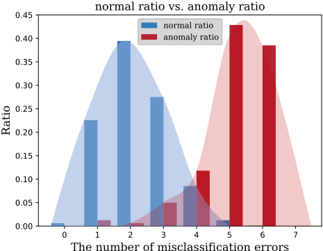
Inspired by approaches in image anomaly detection [Golan and El-Yaniv, 2018], we formulate a hypothesis that the higher the probability of misclassifying perturbation types, the higher the probability of anomalies. In other words, by incorporating an augmentation type recognizer, samples with lower recognition rates are more likely to be anomalies. We proved the correctness of this assumption by designing a classifier to recognize anomalous augmented classes. As shown in Figure 1, we observed that as the number of anomaly detection errors by the classifier increases, the proportion of normal samples decreases while the proportion of anomalous samples increases. In other words, the classifier finds it more difficult to classify perturbed anomalies. On the other hand, existing contrastive learning methods adjust distances to positive and negative samples but neglect class information when selecting negative samples. This can cause samples from the same class to drift apart, causing class collapse [Chuang et al., 2020] and poor representations. To counter this, we integrate class labels into our contrastive learning loss, yielding enhanced model representations and improved performance.
In this paper, we propose a novel Perturbation Guiding Contrastive Representation Learning for Time Series Anomaly Detection method. The approach addresses the issue of class information loss in traditional time series contrastive learning. By introducing the concept of augmentation classification, originally applied in image contrastive learning, to time series data, we have validated its feasibility in aiding anomaly detection. Moreover, we have designed a novel loss function to prevent class collapse, a common problem in contrastive learning. This combination of innovations has resulted in a significant improvement in the performance of anomaly detection for time series data. In a word, our contributions of this paper can be summarized as follow:
- We propose a novel Perturbation Guiding Contrastive Representation Learning for Time Series Anomaly Detection (PCRTA) model. Our model leverages various types of perturbations to train a classification network for generating pseudo-labels. These pseudo-labels are utilized in the selection of positive and negative samples in the contrastive learning network. This approach enhances the discriminative nature of the learned representations, resulting in more robust performance.
- To address the sensitivity and low robustness of contrastive learning to specific perturbation functions, we introduce a variety of data perturbation techniques. Moreover, we integrate a classifier to learn perturbationbased classification and generate pseudo-labels. This augmentation of the learning process enhances the model's ability to adapt to different types of anomalies, improving its overall robustness.
- To tackle the class collapse issue, we leverage the pseudo-labels generated by the classifier. By incorporating key insights from anomaly detection, we refine the selection strategy in contrastive learning and devise a novel contrastive loss function. The perturbation guiding contrastive learning network results in the model producing representations that are more distinct and discriminative, enhancing its ability to differentiate between different classes.
2 RelatedWork
In the section, we briefly review the commonly used methods for anomaly detection on time series data and the application of contrastive learning in time series.
2.1 Anomaly Detection
Anomaly detection is a critical task in various domains to identify rare and abnormal instances in the data. Traditional anomaly detection methods include density-based approaches such as Local Outliers Factor (LOF) [Breunig et al., 2000], distance-based approaches like K-Nearest Neighbors (KNN) [Hautamaki et al., 2004], and linear model-based methods like Principal Component Analysis (PCA) [Patcha and Park, 2007]. A survey [Gupta et al., 2013] summarizes traditional methods for time series anomaly detection. More recently, deep learning has become the mainstream approach for time series anomaly detection. Deep learning models utilize single-class generative models to encode input data, make predictions for future data, and perform contrastive or feature extraction-based processing to identify anomalies. The core idea of these methods lies in implicitly modeling normal patterns and behaviors through the principles of restoration or prediction. By designing various advanced network architectures and novel reconstruction/prediction learning objectives, researchers have successfully improved the performance of time series anomaly detection models. Many studies have focused on capturing more comprehensive dependencies by utilizing variational Autoencoders [Li et al., 2021; Su et al., 2019], graph neural networks [Deng and Hooi, 2021], and Transformer [Tuli et al., 2022; Jiehui Xu and Long, 2022]. However, our goal is to leverage the idea of contrastive learning to process time series features and extract embeddings that can better capture temporal patterns and distinguish anomalies.
2.2 Contrastive Learning
In recent years, contrastive learning has been extensively used in both supervised and unsupervised representation learning. The core idea of contrastive learning is to minimize the contrastive loss [Hadsell et al., 2006], which involves bringing positive sample pairs closer and pushing negative sample pairs further apart, in order to obtain the discriminative space. In supervised learning, contrastive learning is commonly used for deep metric learning [Schroff et al., 2015]. Recently, self-supervised contrastive learning has achieved state-of-the-art performance on downstream visual recognition tasks. Classic pretext tasks such as data augmentations used in SimCLR [Chen et al., 2020] and MoCo [He et al., 2020]. In recent years, there has been a growing interest in applying contrastive learning to time series data [Oord et al., 2018; Eldele et al., 2021; Sana Tonekaboni and Goldenberg, 2021]. Time series contrastive learning trains a feature extractor using multinomial logistic regression to distinguish between different segments in time series data [Hyvarinen and Morioka, 2016]. However one challenge in contrastive learning is the selection of positive and negative samples, which can lead to cases where samples from the same class are mistakenly treated as negative samples, resulting in class collapse and ineffective feature representations. The proposed method introduces a new loss function that incorporates class information, mitigating class collapse and improving the efficiency of the model.
3 Proposed Framework
In this section, we will elaborate the proposed PCRTA model, the network architecture of which is presented in Figure 2.
3.1 Notations and ProblemDefinition
In this paper, our time series dataset observed fromD sensors during time N as X = ⟨x1, x2, · · · , xN⟩ , xt ∈ RD . When D > 1, the dataset X is referred to as a multivariate time series, and the dataset is simplified to a univariate time series if D = 1. Our unsupervised time series anomaly detection f can extract informative embeddings from samples without relying on any pre-existing label information and compute anomaly scores using LOF method [Breunig et al., 2000], i.e., f : X → R. Higher anomaly scores indicate a higher likelihood of being anomalies.
For modeling time series, we adopt a common practice found in most deep time series anomaly detection methods [Campos et al., 2021; Su et al., 2019; Tuli et al., 2022], which involves considering the local contextual window for each observation to model their temporal dependencies. Specifically, we employ a sliding window of length l and stride r to transform the training set into a collection of subsequences denoted as S = {s1, s1+r, · · · }, where st = ⟨xt, xt+1, · · · , xt+l-1⟩. This approach captures the temporal patterns within each subsequence and forms the foundation for our time series modeling. During the inference phase, the test dataset is also divided into subsequences using the same window length l, with a sliding step of 1. The anomaly detection model assesses the anomaly level for each subsequence and assigns an anomaly score to the last timestamp of each subsequence. To obtain the final list of anomaly scores, we pad the initial l - 1 timestamps with zeros. This process ensures that each subsequence is evaluated and assigned an anomaly score, facilitating the identification of anomalies in the time series data.
3.2 Overall Framework
The overall framework PCRTA is shown in Figure 2. We employ a temporal modeling network ϕ to capture temporal correlations and interactions among intrinsic variables. After comparing various feature extraction methods [Zeng et al., 2023], we opt for Temporal Convolutional Networks (TCN) [Bai et al., 2018] as the temporal modeling module for PCRTA. In contrast to conventional RNN-based architectures, TCN utilizes distinctive convolutional kernels that can more swiftly and efficiently extract time-correlated information, resulting in a more effective representation of temporal dependencies within the data, whole representation process can be denoted as ϕ(·). We devised a multi-classification network to learn the sample augmentation strategies. Given that the labels for these augmentation strategies are known, our classification network achieves favorable outcomes guided by the cross-entropy loss Lmul. Consequently, we derive pseudo-labels to guide the contrastive learning network, thereby enhancing the quality of learned representations. Subsequently, we formulated a contrastive learning network. Leveraging the pseudo-labels derived from the multiclassification network, we selected positive and negative samples. Guided by our newly designed contrastive learning loss Lcon, we aimed to bring the features extracted from TCN closer for positive samples and farther for negative samples. This process yielded representations endowed with enhanced discriminative capability. The final computation of the loss function is as follows:
where α is a parameter used to adjust the weights of the contrastive learning network.
3.3 Perturbation Classification Network
PCRTA aims to leverage various perturbation techniques using the concept of learning pseudo-labels to enhance its robustness. Simultaneously, we draw inspiration from viewpoints in image anomaly detection [Golan and El-Yaniv, 2018]: augmentations applied to anomaly data should make it harder for a multi-classifier to discern the augmented category. To achieve this, we define data perturbation δ as specific operations that modify the input time series subsequence s based on the definitions and characteristics of the three fundamental types of time series anomalies (i.e., point anomalies, contextual anomalies, and collective anomalies). This results in a new subsequence s′ , which incorporates the genuine anomalous behaviors of the time series and s and s′ maintain the same shape.
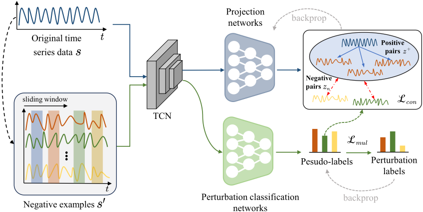
- δ(I,γ) (s): Data augmentation is applied to the last observation of input subsequence s by randomly replacing selected data values with a global extremum value γ, generating a new subsequence with point anomalies.
- δ(II,γ) (s): We augment data by replacing dimensions in the final observation of input subsequence s with an offset γ based on the average of the preceding k values, generating contextual anomalies with a default k of 10.
- δ(III,γ) (s): We augment data by randomly selecting dimensions within a segment of the input subsequence s and replacing the chosen values with the outlier value γ. This creates collective anomalies.
In practice, each of the aforementioned operations employs two γ values to simulate two extreme anomalies. Due to the preprocessing step where time series data is normalized to the range [0, 1], we use γ = +2, -2 in δI, γ = +0.5, -0.5 in δII, γ = 1.0 in δIII. Pool Ω is defined which contains six data augmentations functions and function without augmentation δ0, i.e.,
These six perturbation functions effectively emulate genuine anomalies present in time series data. After augmentation, the augmented data is assigned labels ranging from the first class to the sixth class, representing the augmentation types, while the original non-augmented data is assigned the label of class 0. To make multi-classification network learn pseudolabels, we utilize the cross-entropy loss function to train the classification network:
where N is the number of augmentations Naug + 1 since the non-augmented original data corresponds to the first class.
After learning pseudo-labels through the perturbation classification network, we feed this class information Π into the contrastive learning network. It serves as the basis for selecting positive and negative samples within the contrastive learning framework.
3.4 Perturbation Guiding Contrastive Network
The high dimensionality of the data significantly affects its distribution, resulting in a hyper-ellipsoidal shape rather than a hyper-spherical one. Proposition 1 provides evidence of this. Choosing positive and negative samples under nonnormal data distribution is inaccurate. Therefore, we designed a projection network to project high-dimensional data into a low-dimensional space. We perform positive and negative sample selection on the compacted features.
Proposition 1. Let U be a χ2 statistic with D dimension, for any positive σ, the following inequality holds:
The proof of Proposition 1 can be found in the appendix. According to Proposition 1, the probability of having a compact distribution decreases as the dimensionality of the vector increases. Since the embeddings produced by TCN have high dimensions, to address this issue, we developed a projection network Ψ to reduce the embedding dimensions and improve the representation capability.
Subsequently, we selected positive and negative samples based on the class information Π provided by the classification network. We computed the normalized dot product between pairs of vectors zi and zj within the same class πc.
Then, we select the top k normalized dot products in Eq. 7, gk denotes the indices of top-k values among its input. We use Z + i to denote the postive sample set of zi.
Lastly, for vector zi ∈ πc, all vectors from different classes zn /∈ πc are treated as negative samples. This leads to the construction of the following contrastive learning loss function:
where C is the total number of classes, exp(zT a zb/τ) is the function which measures the similarity of za and zb, and the temperature parameter τ controls the distribution of similarity scores.
In the perturbation guiding contrastive learning network, we employ pseudo-labels obtained from the classification network rather than using the true labels that were originally known. This approach is driven by our core concept that augmenting anomalies is more prone to misclassification compared to normal data. Consequently, when the accuracy of the classifier reaches a higher level, selecting positive samples within the same class and negative samples from different classes becomes more accurate. Due to the tendency for anomalous samples to be assigned to different classes as the model converges, the perturbation guiding contrastive learning network drives a greater separation between normal and anomaly instances. This leads to the extraction of more discriminative representations that effectively capture the distinctions between normal and anomalous patterns.
4 Experimental Results
In this section, we will first present the experimental setup. Subsequently, we will proceed with a series of experiments to assess the effectiveness of the model, its generalization capabilities, robustness, and ablation studies.
4.1 Preliminary
Datasets and Compared Methods. Six real datasets showed in Table 1 for time series anomaly detection are adopted, including WaQ, DSADS, Epilepsy, ASD, SMD 1 , and SWaT[Zhang et al., 2022; Xu et al., 2024]. D means the dimension, #anmo(ratio) is the size of the anomaly and ratio in the testing set, and #seqs is the number of time series sequences in each dataset. We compare PCRTA to the 13 traditional and deep learning anomaly detection methods, including OCSVM [Manevitz and Yousef, 2001], GOAD [Bergman and Hoshen, 2020], ECOD [Li et al., 2022], LSTM-ED [Malhotra et al., 2016], Tcn-ED [Garg et al., 2021], DSVDD [Ruff et al., 2018], MSCRED [Zhang et al., 2019], Omni [Su et al., 2019], USAD [Audibert et al., 2020], GDN [Deng and Hooi, 2021], NeuTraL [Qiu et al., 2021], TranAD [Tuli et al., 2022], and COUTA [Xu et al., 2024]. As a result, the aforementioned list of competitors effectively represents the stateof-the-art performance in the field of time series anomaly detection research.
1 As analysed in the research [Wu and Keogh, 2021], the data quality of some entities in SMD may be flawed. Therefore, we removed these defective entities and retained three entities (machine
3-1, machine 3-9 and machine 3-11)
| Datasets | Training size | Testing size | D | #anom(ratio) | #seqs |
|---|---|---|---|---|---|
| WaQ | 138,521 | 115,086 | 11 | 2,329(0.9%) | 1 |
| DSADS | 85,500 | 57,000 | 47 | 9000(6.3%) | 8 |
| Epilepsy | 33,784 | 22,866 | 5 | 5,768(10.2%) | 1 |
| ASD | 8,528 | 4,320 | 19 | 199(1.5%) | 12 |
| SMD | 28,703 | 28,703 | 38 | 270(0.5%) | 3 |
| SWaT | 475,200 | 449,919 | 51 | 54,584(5.9%) | 1 |
EvaluationMetrics. Following prior work [Audibert et al., 2020; Campos et al., 2021; Su et al., 2019; Tuli et al., 2022; Xu et al., 2024], we use the best F1-Score and the Area Under the Precision-Recall Curve (AUC-PR). F1 = 2 ∗ P rec∗Rec Prec+Rec , where Prec = TP TP+FP and Rec = TP TP+FN , and TP, TN, FP, FN are denote the numbers of true positives, true negatives, false positives, and false negatives. These metrics are suitable for imbalanced data, where the optimal F1 score represents the best-case scenario, and AUC-PR represents the average case in less ideal conditions. We enumerate all possible thresholds (i.e., scores for each timestamp) and compute corresponding precision and recall scores. The optimal F1 can then be obtained, and AUC-PR is calculated using the average precision score. The range of these performance evaluation metrics is from 0 to 1, with higher values indicating better performance.
Experimental Setup. The WaQ, Epilepsy, DSADS, ASD, SMD, and SWaT datasets have been widely used as benchmark datasets in previous literature [Lai et al., 2021; Xu et al., 2024; Campos et al., 2021; Deng and Hooi, 2021; Li et al., 2021; Su et al., 2019; Tuli et al., 2022]. We use a stride of 1 for ASD and SMD, and 100 and 5 for the larger datasets SWaT and WaQ, respectively. For Epilepsy and DSADS, their original data formats are collections of partitioned time series, hence no sliding window is needed. In PCRTA, the TCN ϕ employs a kernel size of 2 and a single hidden layer with the default setting of 16 neural units. We train models for up to 100 epochs, and the weight factor α of the contrastive network is set to 0.2 by default. We choose k = 5 as the parameter for selecting positive samples using nearest neighbors. All the experiments are executed at a workstation with the Intel(R) Xeon(R) Gold 6248R 3.00GHz CPU and NVIDIA TITAN Xp GPU with 10GB RAM, running on the Ubuntu 20.04 operating system.
4.2 Anomaly Detection
We apply the LOF algorithm to compute anomaly scores for the representations obtained from the well-trained perturbation guiding contrastive learning network. For each sample si, we calculate the average score from the 7 representations generated by the 6 augmentation strategies and the original representation.
| Method | WaQ | DSADS | Epilepsy | |||
|---|---|---|---|---|---|---|
| F1 | AUC-PR | F1 | AUC-PR | F1 | AUC-PR | |
| OCSVM | 0.732±0.000 | 0.666±0.000 | 0.807±0.000 | 0.753±0.000 | 0.781±0.000 | 0.708±0.000 |
| GOAD | 0.739±0.052 | 0.685±0.034 | 0.723±0.014 | 0.676±0.015 | 0.554±0.147 | 0.530±0.128 |
| ECOD | 0.676±0.000 | 0.716±0.000 | 0.923±0.000 | 0.941±0.000 | 0.785±0.000 | 0.763±0.000 |
| LSTM-ED | 0.759±0.006 | 0.714±0.018 | 0.865±0.011 | 0.902±0.005 | 0.802±0.012 | 0.784±0.012 |
| Tcn-ED | 0.707±0.082 | 0.658±0.090 | 0.850±0.021 | 0.868±0.023 | 0.758±0.011 | 0.763±0.008 |
| DSVDD | 0.519±0.038 | 0.410±0.043 | 0.751±0.057 | 0.690±0.078 | 0.686±0.040 | 0.555±0.069 |
| MSCRED | 0.717±0.007 | 0.644±0.016 | 0.657±0.029 | 0.659±0.062 | 0.640±0.017 | 0.604±0.023 |
| Omni | 0.738±0.018 | 0.714±0.023 | 0.867±0.018 | 0.914±0.015 | 0.811±0.027 | 0.780±0.054 |
| USAD | 0.666±0.049 | 0.611±0.044 | 0.733±0.041 | 0.713±0.065 | 0.663±0.009 | 0.541±0.038 |
| GDN | 0.640±0.052 | 0.659±0.043 | 0.795±0.022 | 0.728±0.024 | 0.783±0.010 | 0.789±0.010 |
| NeuTraL | 0.681±0.085 | 0.616±0.111 | 0.534±0.035 | 0.490±0.045 | 0.739±0.075 | 0.729±0.111 |
| TranAD | 0.755±0.010 | 0.729±0.017 | 0.730±0.114 | 0.690±0.158 | 0.776±0.008 | 0.734±0.012 |
| COUTA | 0.781±0.013 | 0.714±0.006 | 0.926±0.029 | 0.942±0.020 | 0.830±0.053 | 0.823±0.086 |
| PCRTA | 0.784±0.007 | 0.794±0.002 | 0.943±0.017 | 0.960±0.019 | 0.934±0.015 | 0.964±0.006 |
| Method | ASD | SMD | SWaT | |||
| F1 | AUC-PR | F1 | AUC-PR | F1 | AUC-PR | |
| OCSVM | 0.625±0.000 | 0.540±0.000 | 0.761±0.000 | 0.664±0.000 | 0.839±0.000 | 0.804±0.000 |
| GOAD | 0.827±0.025 | 0.834±0.023 | 0.975±0.019 | 0.981±0.013 | 0.831±0.003 | 0.799±0.005 |
| ECOD | 0.589±0.000 | 0.527±0.000 | 0.755±0.000 | 0.724±0.000 | 0.849±0.000 | 0.899±0.000 |
| LSTM-ED | 0.807±0.013 | 0.767±0.016 | 0.960±0.000 | 0.955±0.009 | 0.847±0.007 | 0.848±0.005 |
| Tcn-ED | 0.853±0.015 | 0.862±0.019 | 0.848±0.050 | 0.881±0.036 | 0.843±0.011 | 0.846±0.003 |
| DSVDD | 0.691±0.014 | 0.671±0.017 | 0.682±0.012 | 0.621±0.033 | 0.829±0.002 | 0.811±0.003 |
| MSCRED | 0.766±0.036 | 0.756±0.050 | 0.628±0.031 | 0.536±0.049 | OOM | OOM |
| Omni | 0.810±0.044 | 0.789±0.063 | 0.954±0.006 | 0.928±0.011 | 0.845±0.012 | 0.841±0.008 |
| USAD | 0.595±0.033 | 0.510±0.035 | 0.744±0.006 | 0.658±0.006 | 0.835±0.000 | 0.808±0.000 |
| GDN | 0.801±0.034 | 0.779±0.042 | 0.939±0.015 | 0.959±0.016 | 0.846±0.025 | 0.885±0.036 |
| NeuTraL | 0.627±0.047 | 0.592±0.045 | 0.770±0.050 | 0.746±0.067 | 0.862±0.023 | 0.850±0.026 |
| TranAD | 0.899±0.020 | 0.915±0.018 | 0.761±0.001 | 0.662±0.003 | 0.831±0.009 | 0.810±0.007 |
| COUTA | 0.942±0.031 | 0.955±0.030 | 0.980±0.018 | 0.984±0.015 | 0.886±0.022 | 0.900±0.017 |
| PCRTA | 0.927±0.080 | 0.933±0.094 | 0.987±0.002 | 0.988±0.001 | 0.978±0.004 | 0.996±0.001 |
(9)
where zaug is embeddings of the augmentations Ω(si), this culminates in the ultimate anomaly score for the sample, offering a comprehensive evaluation of its anomalousness.
As shown in Table 2, PCRTA consistently outperforms or matches other methods in time series anomaly detection. PCRTA achieves top results on five datasets and second-best on one, with remarkable gains on the Epilepsy dataset: a 13% increase in F1 score and a 17% rise in AUC-PR. TranAD, GDN, and COUTA demonstrate strong detection. TranAD utilizes a Transformer and diverse training, GDN employs graph neural networks, and COUTA introduces novel goals and data perturbation. However, TranAD's complexity may lead to overfitting on simpler datasets. Basic architectures like LSTM-ED and Tcn-ED perform well. For SWaT, favoring one-class models due to its normal training and anomaly test data. In contrast, COUTA excels on noisy datasets using introduced anomaly information. PCRTA surpasses by incorporating perturbation type class info and harder-to-detect anomaly concepts via augmentation.
4.3 Visualisation Experiment
In this section, we use t-distributed stochastic neighbor em-
bedding (t-SNE) [Van der Maaten and Hinton, 2008] to visu-
alize whether the representations learned by our model on the
Epilepsy dataset are discriminative. Epilepsy seizure dataset
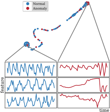
(Epilepsy) is collected from a triaxial accelerometer placed on the dominant wrist. Participants were instructed to perform four different activities, with epileptic seizures defined as the abnormal category and the other three activities, walking, running, and sawing, as normal data. In Figure 3, blue and red colors represent normal and abnormal samples, respectively. While there are some anomalies that are close to normal samples, a distinct cluster of most abnormal samples is formed in the upper right corner, far from the cluster formed by normal samples in the lower left corner.
4.4 Generalization Ability
Due to the model's ability to learn from various perturbation methods, we show improved robustness when dealing with different types of anomalies coexisting within a single dataset. Following a fine-grained categorization of time series anomalies [Lai et al., 2021], we constructed a synthetic dataset containing multiple types of anomalies and conducted a comparison with single-class generative models.
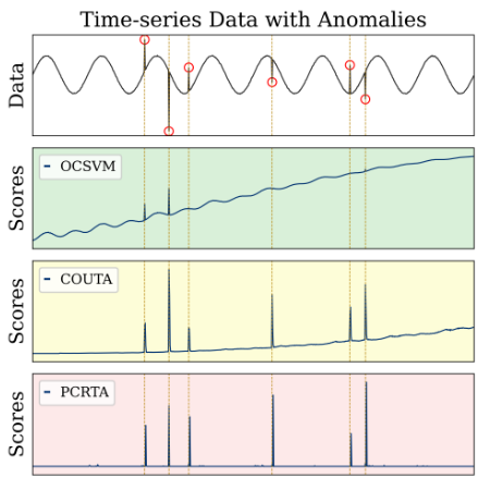
In Figure 4, the top section represents the synthetic dataset, while the bottom section displays the anomaly scores obtained by different models when tested on the synthetic dataset. The performance of OCSVM degrades over time, accumulating errors in the time series data and leading to increasing anomaly scores. COUTA, although incorporating anomaly information, lacks robustness by failing to discriminate between different perturbation effects, and therefore there is a small increase in the anomaly scores. These oneclass learning models excel at detecting different anomalies, but some methods show fluctuating scores, making analysis difficult. In contrast, PCRTA excels at effectively handling perturbation classes, yielding high, stable anomaly scores for anomalies and normal instances.
4.5 Ablation Study
We perform ablation experiments on the two main components of our model. We employ three ablation variants: replacing pseudo-labels from the classification network with ground truth, freezing the parameters of the classification network, and freezing the parameters of the contrastive network. These variants correspond to removing pseudo-labels, classification learning loss as Eq. 3, and contrastive learning loss as
| WaQ | DSADS | Epilepsy | ||||
|---|---|---|---|---|---|---|
| Method | F1 | AUC | F1 | AUC | F1 | AUC |
| ground truth | 0.73 | 0.75 | 0.93 | 0.94 | 0.89 | 0.91 |
| w/o Lmul(3) | 0.67 | 0.68 | 0.61 | 0.55 | 0.92 | 0.94 |
| w/o Lcon(8) | 0.74 | 0.74 | 0.90 | 0.88 | 0.87 | 0.91 |
| PCRTA | 0.78↑ | 0.79↑ | 0.94↑ | 0.96↑ | 0.93↑ | 0.96↑ |
Eq. 8 from the model. The comparative analysis of PCRTA and its variants reveals that the superiority of PCRTA on the majority of the 26 sequences from six real-world datasets can be attributed to the innovative concept of utilizing the classification network, the contrastive network, and the classification network-guided contrastive network.
From Table 3, we can observe the results of the ablation experiments. The performance of the contrastive network guided by ground truth is inferior to PCRTA. Pseudo-labels offers several advantages: 1. In our selection strategy for positive and negative samples, samples with a high number of perturbation type misclassifications are considered anomalies. Pseudo-labels prevent the representations of anomalies from being selected, which would not be achievable with true labels. 2. For model training, using ground truth at the beginning of the training process would lead to minimal variation in positive and negative samples within the contrastive network, making the model susceptible to early convergence to local optima and hindering further training. 3. One of the core ideas of PCRTA is based on the assumption of low perturbation recognition rates in anomalies. Thus, a perturbation classification network is needed for anomaly selection.
5 Conclusion
In this paper, we propose our Perturbation Guiding Contrastive Representation Learning for Time Series Anomaly Detection (PCRTA), which combines the power of contrastive learning and classification-guided augmentation to enhance the performance of time series anomaly detection. Through extensive experiments on six real-world datasets, PCRTA consistently outperformed a range of state-of-the-art competitors, demonstrating its effectiveness and robustness. In the future, we can consider additional architectures to enhance the performance and practicality of the model.
@inproceedings{ijcai2024p548,
  title     = {Perturbation Guiding Contrastive Representation Learning for Time Series Anomaly Detection},
  author    = {Tang, Liaoyuan and Wang, Zheng and He, Guanxiong and Wang, Rong and Nie, Feiping},
  booktitle = {Proceedings of the Thirty-Third International Joint Conference on
               Artificial Intelligence, {IJCAI-24}},
  publisher = {International Joint Conferences on Artificial Intelligence Organization},
  editor    = {Kate Larson},
  pages     = {4955--4963},
  year      = {2024},
  month     = {8},
  note      = {Main Track},
  doi       = {10.24963/ijcai.2024/548},
  url       = {https://doi.org/10.24963/ijcai.2024/548},
}
TY - CPAPER TI - Perturbation Guiding Contrastive Representation Learning for Time Series Anomaly Detection AU - Tang, Liaoyuan AU - Wang, Zheng AU - He, Guanxiong AU - Wang, Rong AU - Nie, Feiping T2 - Proceedings of the Thirty-Third International Joint Conference on Artificial Intelligence, IJCAI-24 PB - International Joint Conferences on Artificial Intelligence Organization PY - 2024 SP - 4955 EP - 4963 DO - 10.24963/ijcai.2024/548 UR - https://doi.org/10.24963/ijcai.2024/548 ER -Copied
Machine-readable versions of this paper, for tools and AI agents:





