
LSPAN: Spectrally Localized Augmentation for Graph Consistency Learning
Proceedings of the Thirty-Third International Joint Conference on Artificial Intelligence. Main Track. Pages 5462-5470.
https://doi.org/10.24963/ijcai.2024/604
Keywords
- Machine Learning: ML: Active learning
- Machine Learning: ML: Classification
- Machine Learning: ML: Semi-supervised learning
- Machine Learning: ML: Multi-task and transfer learning
Abstract
Graph-based consistency principle has been successfully applied to many semi-supervised problems in machine learning. Its performance largely depends on the quality of augmented graphs, which has been recently proven that revealing graph properties and maintaining the invariance of graphs are crucial for good performance. However, existing topology- or feature-based augmentation methods are spectrally non-localized -- important spectrums are disturbed throughout the entire frequency range, and their invariance may not be well preserved. Efforts on this issue remain to be limited. This paper proposes a simple yet effective model called Localized SPectral AugmentatioN (LSPAN), which perturbs a concentrated part of graph spectrum with equivalent intensity using Fourier orthogonality, so as to enhance graph spectrum preservation as well as model prediction. Moreover, it also avoids the significant training time of inverse Fourier transform. Extensive empirical evaluation on real-world datasets clearly shows the performance gain of spectrally localized augmentation, as well as its good convergence and efficiency compared to existing graph methods.
- [Abu-El-Haija et al., 2019] Sami Abu-El-Haija, Bryan Per- ozzi, Amol Kapoor, Nazanin Alipourfard, Kristina Lerman, Hrayr Harutyunyan, Greg Ver Steeg, and Aram Galstyan. Mixhop: Higher-order graph convolutional architectures via sparsified neighborhood mixing. In Proceedings of the International Conference on Machine Learning, pages 21-29, 2019.
- [Berthelot et al., 2019] David Berthelot, Nicholas Carlini, Ian Goodfellow, Nicolas Papernot, Avital Oliver, and Colin A Raffel. Mixmatch: A holistic approach to semi- supervised learning. In Advances in Neural Information Processing Systems, pages 5050-5060, 2019.
- [Bo et al., 2022] Deyu Bo, Binbin Hu, Xiao Wang, Zhiqiang Zhang, Chuan Shi, and Jun Zhou. Regularizing graph neu- ral networks via consistency-diversity graph augmentations. In Proceedings of the AAAI Conference on Artificial Intelli- gence, pages 3913-3921, 2022.
- [Chen et al., 2020] Deli Chen, Yankai Lin, Wei Li, Peng Li, Jie Zhou, and Xu Sun. Measuring and relieving the over- smoothing problem for graph neural networks from the topological view. In Proceedings of the AAAI Conference on Artificial Intelligence, pages 3438-3445, 2020.
- [Chien et al., 2021] Eli Chien, Jianhao Peng, Pan Li, and Ol- gica Milenkovic. Adaptive universal generalized pagerank graph neural network. In Proceedings of the International Conference on Learning Representations, 2021.
- [Chung, 1997] Fan RK Chung. Spectral graph theory, vol- ume 92. American Mathematical Soc., 1997.
- [Defferrard et al., 2016] Michaël Defferrard, Xavier Bresson, and Pierre Vandergheynst. Convolutional neural networks on graphs with fast localized spectral filtering. In Advances in Neural Information Processing Systems, pages 3844- 3852, 2016.
- [Deng et al., 2019] Zhijie Deng, Yinpeng Dong, and Jun Zhu. Batch virtual adversarial training for graph convolutional networks. arXiv preprint arXiv:1902.09192, 2019.
- [Ding et al., 2022] Kaize Ding, Zhe Xu, Hanghang Tong, and Huan Liu. Data augmentation for deep graph learning: A survey. ACM SIGKDD Explorations Newsletter, 24(2):61- 77, 2022.
- [Feng et al., 2019] Fuli Feng, Xiangnan He, Jie Tang, and Tat-Seng Chua. Graph adversarial training: Dynamically regularizing based on graph structure. IEEE Transactions on Knowledge and Data Engineering, 33(6):2493-2504, 2019.
- [Feng et al., 2020] Wenzheng Feng, Jie Zhang, Yuxiao Dong, Yu Han, Huanbo Luan, Qian Xu, Qiang Yang, Evgeny Khar- lamov, and Jie Tang. Graph random neural networks for semi-supervised learning on graphs. In Advances in Neu- ral Information Processing Systems, pages 22092-22103, 2020.
- [Fout et al., 2017] Alex Fout, Jonathon Byrd, Basir Shariat, and Asa Ben-Hur. Protein interface prediction using graph convolutional networks. In Advances in Neural Information Processing Systems, pages 6530-6539, 2017.
- [Gao and Ji, 2019] Hongyang Gao and Shuiwang Ji. Graph u-nets. In Proceedings of the International Conference on Machine Learning, pages 2083-2092, 2019.
- [Ghose et al., 2023] Amur Ghose, Yingxue Zhang, Jianye Hao, and Mark Coates. Spectral augmentations for graph contrastive learning. In Proceedings of the International Conference on Artificial Intelligence and Statistics, pages 11213-11266, 2023.
- [Gori et al., 2005] Marco Gori, Gabriele Monfardini, and Franco Scarselli. A new model for learning in graph do- mains. In Proceedings of the 2005 IEEE International Joint Conference on Neural Networks, pages 729-734, 2005.
- [Hamilton et al., 2017] Will Hamilton, Zhitao Ying, and Jure Leskovec. Inductive representation learning on large graphs. In Advances in Neural Information Processing Systems, pages 1024-1034, 2017.
- [Hammond et al., 2013] David K Hammond, Yaniv Gur, and Chris R Johnson. Graph diffusion distance: A difference measure for weighted graphs based on the graph lapla- cian exponential kernel. In Proceedings of the 2013 IEEE Global Conference on Signal and Information Processing, pages 419-422, 2013.
- [Huang et al., 2017] Xiao Huang, Jundong Li, and Xia Hu. Label informed attributed network embedding. In Proceed- ings of the Tenth ACM International Conference on Web Search and Data Mining, pages 731-739, 2017.
- [Kahale, 1995] Nabil Kahale. Eigenvalues and expansion of regular graphs. Journal of the ACM (JACM), 42(5):1091- 1106, 1995.
- [Kipf and Welling, 2017] Thomas N Kipf and Max Welling. Semi-supervised classification with graph convolutional networks. In Proceedings of the International Conference on Learning Representations, 2017.
- [Kong et al., 2020] Kezhi Kong, Guohao Li, Mucong Ding, Zuxuan Wu, Chen Zhu, Bernard Ghanem, Gavin Tay- lor, and Tom Goldstein. Flag: Adversarial data aug- mentation for graph neural networks. arXiv preprint arXiv:2010.09891, 2020.
- [Lee et al., 2014] James R Lee, Shayan Oveis Gharan, and Luca Trevisan. Multiway spectral partitioning and higher- order cheeger inequalities. Journal of the ACM (JACM), 61(6):1-30, 2014.
- [Li et al., 2019] Yu-Feng Li, Lan-Zhe Guo, and Zhi-Hua Zhou. Towards safe weakly supervised learning. IEEE Transactions on Pattern Analysis and Machine Intelligence, 43(1):334-346, 2019.
- [Lin et al., 2023] Lu Lin, Jinghui Chen, and Hongning Wang. Spectral augmentation for self-supervised learning on graphs. In Proceedings of the International Conference on Learning Representations, 2023.
- [Liu et al., 2022a] Nian Liu, Xiao Wang, Deyu Bo, Chuan Shi, and Jian Pei. Revisiting graph contrastive learning from the perspective of graph spectrum. In Advances in Neural Information Processing Systems, pages 2972-2983, 2022.
- [Liu et al., 2022b] Songtao Liu, Rex Ying, Hanze Dong, Lan- qing Li, Tingyang Xu, Yu Rong, Peilin Zhao, Junzhou Huang, and Dinghao Wu. Local augmentation for graph neural networks. In Proceedings of the International Con- ference on Machine Learning, pages 14054-14072, 2022.
- [Miyato et al., 2018] Takeru Miyato, Shin-ichi Maeda, Masanori Koyama, and Shin Ishii. Virtual adversarial training: a regularization method for supervised and semi-supervised learning. IEEE Transactions on Pattern Analysis and Machine Intelligence, 41(8):1979-1993, 2018.
- [Park et al., 2021] Hyeonjin Park, Seunghun Lee, Sihyeon Kim, Jinyoung Park, Jisu Jeong, Kyung-Min Kim, Jung- Woo Ha, and Hyunwoo J Kim. Metropolis-hastings data augmentation for graph neural networks. In Advances in Neural Information Processing Systems, pages 19010- 19020, 2021.
- [Rong et al., 2020] Yu Rong, Wenbing Huang, Tingyang Xu, and Junzhou Huang. Dropedge: Towards deep graph convo- lutional networks on node classification. In Proceedings of the International Conference on Learning Representations, 2020.
- [Scarselli et al., 2008] Franco Scarselli, Marco Gori, Ah Chung Tsoi, Markus Hagenbuchner, and Gabriele Monfardini. The graph neural network model. IEEE Transactions on Neural Networks, 20(1):61-80, 2008.
- [Shuman et al., 2013] David I Shuman, Sunil K Narang, Pas- cal Frossard, Antonio Ortega, and Pierre Vandergheynst. The emerging field of signal processing on graphs: Ex- tending high-dimensional data analysis to networks and other irregular domains. IEEE Signal Processing Maga- zine, 30(3):83-98, 2013.
- [Veličković et al., 2018] Petar Veličković, Guillem Cucurull, Arantxa Casanova, Adriana Romero, Pietro Liò, and Yoshua Bengio. Graph attention networks. In Proceedings of the International Conference on Learning Representa- tions, 2018.
- [Wang et al., 2020] Haibo Wang, Chuan Zhou, Xin Chen, Jia Wu, Shirui Pan, and Jilong Wang. Graph stochastic neural networks for semi-supervised learning. In Advances in Neu- ral Information Processing Systems, pages 19839-19848, 2020.
- [Wijesinghe and Wang, 2022] Asiri Wijesinghe and Qing Wang. A new perspective on" how graph neural networks go beyond weisfeiler-lehman?". In Proceedings of the In- ternational Conference on Learning Representations, 2022.
- [Wu et al., 2019] Jun Wu, Jingrui He, and Jiejun Xu. Demo- net: Degree-specific graph neural networks for node and graph classification. In Proceedings of the 25th ACM SIGKDD International Conference on Knowledge Discov- ery & Data Mining, pages 406-415, 2019.
- [Wu et al., 2020a] Yongji Wu, Defu Lian, Yiheng Xu, Le Wu, and Enhong Chen. Graph convolutional networks with markov random field reasoning for social spammer detec- tion. In Proceedings of the AAAI Conference on Artificial Intelligence, pages 1054-1061, 2020.
- [Wu et al., 2020b] Zonghan Wu, Shirui Pan, Fengwen Chen, Guodong Long, Chengqi Zhang, and S Yu Philip. A com- prehensive survey on graph neural networks. IEEE Trans- actions on Neural Networks and Learning Systems, 32(1):4- 24, 2020.
- [Yao et al., 2019] Liang Yao, Chengsheng Mao, and Yuan Luo. Graph convolutional networks for text classification. In Proceedings of the AAAI Conference on Artificial Intelli- gence, pages 7370-7377, 2019.
- [Zhang et al., 2019] Yingxue Zhang, Soumyasundar Pal, Mark Coates, and Deniz Ustebay. Bayesian graph con- volutional neural networks for semi-supervised classifica- tion. In Proceedings of the AAAI Conference on Artificial Intelligence, pages 5829-5836, 2019.
- [Zhang et al., 2023] Yifei Zhang, Hao Zhu, Zixing Song, Pi- otr Koniusz, and Irwin King. Spectral feature augmentation for graph contrastive learning and beyond. In Proceedings of the AAAI Conference on Artificial Intelligence, pages 11289-11297, 2023.
- [Zhao et al., 2021] Tong Zhao, Yozen Liu, Leonardo Neves, Oliver Woodford, Meng Jiang, and Neil Shah. Data aug- mentation for graph neural networks. In Proceedings of the AAAI Conference on Artificial Intelligence, pages 11015- 11023, 2021.
- [Zhao et al., 2022] Tong Zhao, Gang Liu, Stephan Günnemann, and Meng Jiang. Graph data augmen- tation for graph machine learning: A survey. arXiv preprint arXiv:2202.08871, 2022.
- [Zhou, 2018] Zhi-Hua Zhou. A brief introduction to weakly supervised learning. National Science Review, 5(1):44-53, 2018.
- [Zhu and Koniusz, 2021] Hao Zhu and Piotr Koniusz. Simple spectral graph convolution. In Proceedings of the Interna- tional Conference on Learning Representations, 2021.
- [Zhu et al., 2003] Xiaojin Zhu, Zoubin Ghahramani, and John D Lafferty. Semi-supervised learning using gaussian fields and harmonic functions. In Proceedings of the Inter- national Conference on Machine Learning, pages 912-919, 2003.
- [Zhu et al., 2021] Dan-Hao Zhu, Xin-Yu Dai, and Jia-Jun Chen. Pre-train and learn: Preserving global information for graph neural networks. Journal of Computer Science and Technology, 36(6):1420-1430, 2021.
References were extracted automatically from the PDF and may contain errors.
Full text extracted automatically from the PDF; figures, tables and equations may differ. The PDF is the version of record.
1 Introduction
Graph machine learning receives considerable attention in recent years due to its ability of exploiting rich information encoded in non-Euclidean data and has been applied to many real-world applications [Fout et al., 2017; Yao et al., 2019; Wu et al., 2020a]. One of the main focuses of this field, graph semi-supervised learning [Zhu et al., 2003; Kipf and Welling, 2017], aims to classify unlabeled nodes in a scarcely labeled graph [Wu et al., 2020b]. However, although Graph Neural Networks (GNNs) [Gori et al., 2005; Scarselli et al., 2008; Kipf and Welling, 2017; Veliˇckovi´c et al., 2018; Hamilton et al., 2017] are introduced to provide powerful solutions for this task, unlabeled nodes that are abundant and informative in practical scenarios [Zhou, 2018; Li et al., 2019; Miyato et al., 2018] are usually not well used - GNNs are trained only over predictions of labeled nodes and the unlabeled nodes are not involved. Recently, graph consistency learning [Park et al., 2021; Bo et al., 2022; Feng et al., 2020] shows a promising framework for utilizing unlabeled nodes by minimizing the predictions divergence of them across different augmented graphs [Zhao et al., 2022; Ding et al., 2022].
∗Corresponding author
Designed for exploiting invariant information with augmented graphs, the performance of graph consistency learning highly relies on the quality of adopted graph augmentation methods. Existing graph augmentation approaches are usually divided into two categories: topology-based approaches [Rong et al., 2020; Zhao et al., 2021; Lin et al., 2023] generate different graph structures by perturbing the adjacency matrix; feature-based approaches [Deng et al., 2019; Feng et al., 2019; Kong et al., 2020; Liu et al., 2022b] perturb node attributes within the feature matrix. In general, previous approaches typically define graph augmentation in the spatial domain (i.e., they work by perturbing either graph structures or node features). Note that although there are recent works like SPAN [Lin et al., 2023] considering spectral information, the spectral knowledge is only used for supervising edge or feature perturbations and they still fall into spatial augmentations.
In this paper, we suggest existing spatial-based augmentation methods can be improved from a new spectral perspective. Specifically, the structure of graph spectrum proves critical in revealing significant graph properties both structurally and semantically [Chung, 1997; Kahale, 1995; Lee et al., 2014; Hammond et al., 2013]. Therefore, preserving the informative spectrum structure is crucial to ensure a good model performance. However, in spatial-domain-based augmentation approaches, the spectrum of an input graph is perturbed at all range of graph frequencies. For example, when an edge is dropped, the spectrum on all Fourier bases can be modified. We define this kind of augmentation as spectrally nonlocalized. In such cases, the relative intensity and location between different spectrum components can be significantly altered and structure of graph spectrum can be largely changed, which may lead to notable information loss in augmented graphs and therefore hinder graph learning. To this end, we hope to design a graph augmentation approach that is able to enhance the preservation of the graph spectrum structure, so as to improve the performance of graph consistency learning.
One promising solution is to keep the majority of graph spectrum unchanged by only perturbing a concentrated part of it, which is named by Localized SPectral AugmentatioN
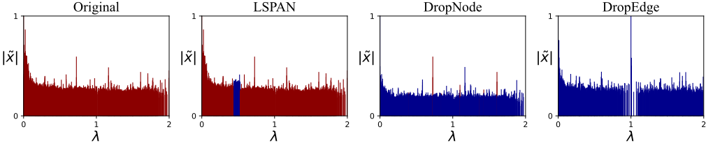
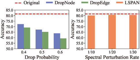
(LSPAN). Specifically, in LSPAN approach, graph spectrum is not perturbed in the entire frequency range. By contrast, only a small localized "block" of spectrum is modified. In this way, the informative graph spectrum is mostly retained and the graph information can be better preserved, which ensures a better generalization performance for model prediction. This is illustrated in Figure 1 - the graph spectrum is only perturbed within a small scope and is mostly retained in LSPAN method, but the overall spectrum structure is largely changed in non-localized ones. Figure 2 shows the prediction accuracy of GCN on original CORA graph, CORA perturbed by non-localized methods and LSPAN (respectively with drop node/edge probability around 0.5 and spectral perturbation rate around 1/20, which are used in prior works [Feng et al., 2020; Liu et al., 2022b] and ours to report final results to ensure fair comparison). We observe that the performance of graph learning decreases significantly with non-localized augmentations while LSPAN still maintains a good performance, which verifies that the graph information is lost much in non-localized augmentations but well preserved in the proposed LSPAN.
To implement LSPAN, we directly define graph augmentation in the spectral domain. To avoid the time-consuming inverse Fourier transform during training, we introduce the Fourier basis orthogonality, which enables LSPAN to be efficiently performed by simple feature concatenation. Extensive empirical evaluation on real-world benchmarks clearly shows the significant performance gain of our method, as well as good convergence properties compared to existing ones.
We summarize our main contributions as follows:
- We identify that existing graph augmentations can cause graph information loss because they are non-localized in spectral domain - graph spectrums that contain important graph information are perturbed over the entire frequency range and their structures can be largely changed.
- We propose a novel spectrally localized augmentation method called LSPAN, which only perturbs the graph spectrum within a small frequency scope and therefore ensures a better preservation of the graph information.
- We conduct extensive empirical studies on six real-world benchmark datasets across four domains, which clearly show the advanced performance of our proposed method.
2 Preliminaries
Notations. Let G = (X,A) be a connected undirected graph with N nodes and E edges. X ∈ RN×F denotes the feature matrix, where F indicates the number of node features. A ∈ {0, 1}N×N denotes the adjacency matrix, where Aij = 1 if edge exists between node i and j and Aij = 0 otherwise. Then, the graph Laplacian is defined as L = D-A ∈ RN×N , where D indicates the diagonal degree matrix, namely Dii = ∑j Aij. The symmetric normalized adjacency matrix is further defined as ˆA = ˜D- 12 ˜A˜D- 12 , where ˜A represents the adjacency matrix for a graph with added self-loops and ˜D is the diagonal degree matrix of ˜A.
Consistency-Based GNN Methods. Consistency-based graph semi-supervised learning [Park et al., 2021; Bo et al., 2022; Feng et al., 2020] provides powerful framework for exploiting unlabeled nodes by minimizing the prediction divergence of them across different augmented graphs G′ = (X′ ,A′ ) [Zhao et al., 2022; Ding et al., 2022], where X′ and A′ indicate the augmented feature and adjacency matrix. They generally expand the loss function as: L = Lsup + γLcon, where Lsup indicates the supervised loss calculated on different graph views, Lcon indicates the consistency regularization loss used for smoothing the label predictions across augmented graph samples and γ controls the strength of it. Augmented graphs are significantly involved in the calculation of Lsup and Lcon. Therefore, the performance of graph consistency learning highly relies on the quality of adopted augmentation approaches. Our work focuses on designing an augmentation method that is spectrally localized and improves the graph spectrum preservation, so as to enhance the model performance. Next, we briefly review the graph spectrum theory.
Introduction to Graph Spectrum. Digital Signal Processing converts a signal into spectral domain and is adopted for graphs by Graph Fourier transform (GFT) [Shuman et al., 2013]. Specifically, In GFT, the real symmetric matrix L is orthogonally diagonalized by: L = UΛUT . We define the eigenvalues {λi}Ni=1 in Λ as graph frequencies (we assume that λ1 ≤ λ2 · · · ≤ λN). They reveal the distribution of graph spectrum and decide where spectrum components are located. We further define the graph Fourier transform as: ˜X=UT X and inverse graph Fourier transform as: X = U˜X, where X indicates the input graph feature matrix and ˜X the feature matrix projected into the spectral domain. In particular, the i-th column ui of U is defined as the Fourier basis at frequency λi and ˜xi = uTi X is the projection of the graph features on this basis, which therefore reveals the strength of spectrum at frequency λi. Overall, frequencies {λi}Ni=1 decide where components of spectrum are located and feature projections {˜xi}Ni=1 reveal the strength of them. The graph spectrum encoded in {λi}Ni=1 and {˜xi}Ni=1 significantly reveals graph properties and is highly desired to be preserved for good learning performance [Chung, 1997; Kahale, 1995; Lee et al., 2014; Hammond et al., 2013].
3 LSPAN: Spectrally Localized Augmentation on Graphs
In this section, we introduce the proposed Localized SPectral AugmentatioN (LSPAN) to preserve important graph spectrum structure for graph consistency learning. Specifically, we first view graph augmentations from the spectral perspective and define spectrally localized graph augmentation based on this. Then, we implement the localized graph augmentation with orthogonality of Fourier bases, which totally avoids the timeconsuming training time Fourier inverse transform and makes our method easily applicable.
3.1 Viewing Graph Augmentation from the Spectral Perspective
To define spectrally localized augmentation on graphs, we first formalize the graph augmentations in the spectral domain by viewing them as perturbations to graph frequencies and feature projections.
Specifically, as mentioned in Section 2, the spectrum of a graph is encode in {λi}Ni=1 and {˜xi}Ni=1 , where {λi}Ni=1 are eigenvalues of graph Laplacian L = D - A and are defined as graph frequencies, which reveal the location distribution of spectrum components. On the other hand, {˜xi}Ni=1 are projections of input graph feature matrix on Fourier bases {ui}Ni=1 , namely ˜xi = uTi X. ui is the i-th eigenvector of graph Laplacian and defined as the Fourier basis at frequency
λi. Therefore, ˜xi is the feature projection on this basis and reveals the strength of spectrum component at frequency λi.
By this, graph augmentations in the spectral domain can be defined by perturbations on graph frequencies {λi}Ni=1 and feature projections {˜xi}Ni=1 as follows:
Definition 1 (Spectral Augmentation on Graphs). Given a graph with frequencies {λi}Ni=1 and feature projections {˜xi}Ni=1 , the spectral augmentation on it is defined as:
where constant ∆λi and vector ∆˜xi denote the perturbations on the i-th graph frequency and i-th feature projection. P is a set of numbers indicating the locations of perturbed spectrum components.
Based on this, spatial graph augmentations can be formalized in spectral domain as follows:
The proofs are deferred to Appendix A. We observe that, feature augmentation only perturbs strength of spectrum components revealed by projections ˜xi while topology augmentation also perturbs locations of spectrum components revealed by frequencies λi. However, regardless of the kind of perturbation, the entire range of spectrum components can be perturbed (i = 1, 2, · · · ,N) and the spectrum structure may deviate from the original one - usually ∆λi ̸= ∆λj and ∆˜xi ̸= ∆˜xj , which means the relative intensity and location of spectrum components can be significantly altered. Therefore, we propose to better retain the spectrum structure by narrowing and localizing the range of perturbation.
3.2 Defining Spectrally Localized Augmentation
To improve the preservation of graph spectrum, we propose to use spectrally localized augmentation where we only perturb a concentrated part of the spectrum. In this way, we restrict the range of perturbable spectrum to a localized "block" and the informative spectral-domain structure is mostly retained. Specifically, the localized augmentation is defined as follows:
Definition 2 (Localized Spectral Augmentation on Graphs). Given a graph with frequencies {λi}Ni=1 and feature projections {˜xi}Ni=1 , the localized spectral augmentation on it is defined as:
where vector ∆˜xi denotes the perturbation on the i-th feature projection.
We ensure m ≥ 1 and m + n ≤ N + 1. As can be seen, in proposed localized augmentation, frequencies {λi}Ni=1 remain unchanged and feature projections {˜xi}Ni=1 are only perturbed within a concentrated frequency range (i ∈ [m, m + n - 1]). In this way, only n spectrum components are perturbed and the structure of graph spectrum is better preserved as shown in Figure 1.
After performing augmentation in the spectral domain, we then transform the perturbed graph back to spatial domain for graph consistency learning. Specifically, we aim to recover the graph G′ with adjacency matrix A′ and feature matrix X′ from augmented frequencies and feature projections {λ′i , ˜x′i }Ni=1 = {AUG(λi, ˜xi)}Ni=1 . As frequencies {λi}Ni=1 remain unchanged, we simply let A′ = A to preserve the graph Laplacian. Then, the feature matrix is recovered by inverse Fourier transform: X′ = U˜X′ . Remind that U is the eigenvector matrix of graph Laplacian, namely L = UΛUT . ˜X′ denotes the augmented feature projection matrix composed of {˜x′i }Ni=1 , namely ˜X′ = [˜x′T 1 , ˜x′T 2 , · · · , ˜x′T N ]T . Overall, we let A′ = A and X′ = U [˜x′T 1 , ˜x′T 2 , · · · , ˜x′T N ]T .
However, in this augmentation, although matrix U and vectors {˜xi}Ni=1 are pre-calculated, the application of Fourier inverse transformX′ =U˜X′ is time-consuming. To address this issue, we simplify the localized augmentation and use the orthogonality of Fourier bases to implement it.
3.3 Implementing Localized Augmentation with Fourier Orthogonality
To avoid time-consuming Fourier inverse transform at training time, we implement localized spectral augmentation with the orthogonality of Fourier bases. By this, the proposed augmentation can be performed by simple feature concatenation in spatial domain and the training time Fourier transform is totally avoided. Specifically, we first redefine the localized augmentation as:
where two simplification tricks are applied. First, the perturbation to feature projection is redefined as (˜xi +∆˜xi) → [˜xi ; T] where [· ; ·] indicates vector or matrix concatenation and the constant T acts as the "temperature" that controls the intensity of perturbation. Second, the spectrum components are perturbed with same intensity constant T, but ∆˜xi ̸= ∆˜xj could happen in previous definitions. This is equivalent to introducing a new graph signal that has and only has components of the same intensity T at frequencies λ = {λm, λm+1, · · · λm+n-1}.
Under this definition, the localized augmentation is actually a perturbation on the feature projection matrix ˜X = UT X by matrix concatenation in the spectral domain, namely:
where α ∈ {0, 1}N represents the introduced new graph signal where αi = 1 if i ∈ [m, m + n - 1] and αi = 0 otherwise. To achieve the spectral augmentation defined in Equation (4) and Equation (5), a graph with adjacency matrix A and feature matrix X is augmented in spatial domain by:
Algorithm 1 Augmentation Phase of LSPAN
Input: Original graph G = (X,A), eigenvectors of graph Laplacian {ui}Ni=1 , parameters m and n, temperature T Output: Augmented graph G′
- 1: Obtain the adjacency matrix: A′ = A.
- 2: Compute the summation of eigenvectors: u′ = (um + um+1 + · · · um+n-1).
- 3: Generate the augmented feature matrix: X′ = [X ; Tu′ ].
- 4: return G′ = (X′ ,A′ )
Specifically, Fourier bases {ui}Ni=1 are eigenvectors of orthogonally diagonalized real symmetric Laplacian matrix. Based on their orthogonality, it can be derived that ∑m+n-1 i=m UT ui = α. By this, the spectral projection of augmented feature matrix in Equation (6) is ˜X′ = UT [X ; T (um + um+1 + · · · um+n-1)] = [ ˜X ; T ∑m+n-1 i=m UT ui] = [ ˜X ; Tα], which is same as the projection ˜X′ defined in Equation (5). This means, by performing the augmentation in Equation (6), the localized spectral augmentation defined in Equation (4) and (5) is achieved. More details of this are covered in Appendix A.
Overall, the proposed LSPAN method augments a graph G = (X,A) by Equation (6), where for the feature matrix, we first compute the summation of eigenvectors {ui}m+n-1 i=m and then perform a matrix concatenation. The adjacency matrix remains unchanged. Details of the LSPAN augmentation method are outlined in Algorithm 1.
Efficiency of LSPAN. Note that the eigenvectors are drawn from the original graph Laplacian and can be pre-calculated. Therefore, during training, only matrix concatenations and vector summations with computational cost of O(N) are required and the time-consuming Fourier inverse transform is totally avoided, which ensures the efficiency of our method. An empirical time analysis is conducted in Appendix C.9.
Placing LSPAN in the Context of Prior Work. Existing augmentations are mainly divided into topology-based [Rong et al., 2020; Zhao et al., 2021; Lin et al., 2023] and feature-based [Deng et al., 2019; Feng et al., 2019; Kong et al., 2020] ones. We suggest that they are spectrally non-localized and may not well preserve the graph information. Note that the recent works [Lin et al., 2023; Liu et al., 2022a; Ghose et al., 2023] also consider spectral information. But they only use the spectral knowledge for supervising edge or feature perturbations and they still fall into spatial augmentation approaches. The work of SFA [Zhang et al., 2023] has a very different underlying principle to ours where the singular values of feature maps are perturbed and the spectrum information is not utilized. Unlike previous works, we directly perturb graph spectrum components in the spectral domain and can control any specific spectrum components, so as to perform strictly localized augmentation.
4 Spectrally Localized Augmentation on Graph Consistency Learning
We apply the proposed LSPAN method to graph consistency learning framework following the work of GRAND [Feng et al., 2020], so as to show our proposal can be easily deployed in graph consistency learning frameworks and show how the proposed spectrally localized augmentation benefits them.
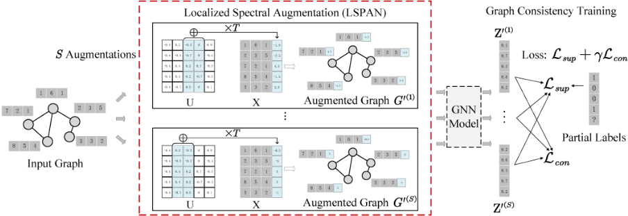
Specifically, given an input graph G with feature matrix X and adjacency matrix A, we first generate S augmented graphs by Equation (6) where T , n are set as hyper-parameters and we randomly choose m from 1 to N - n + 1 for each augmentation. Then, each of the S graphs with augmented feature matrix X′(s) and adjacency matrix A′(s) is fed into a GNN model to obtain corresponding outputs:
where Z′(s) ∈ [0, 1]N×C represents the prediction probabilities on X′(s) and A′(s) with C denoting the number of node classes. The GNN model can be GCN [Kipf and Welling, 2017], GAT [Veliˇckovi´c et al., 2018] or any other state-of-theart methods. For example, in GRAND, a mixed-order propagation model performed by Z = fmlp( 1 K+1 ∑Kk=0 ˆAkX,Θ) is adopted, where ˆA is the symmetric normalized adjacency matrix, fmlp is a two-layer MLP and Θ are parameters. This design eliminates nonlinearity for high-order feature propagation and helps to reduce the over-smoothing risk.
Then, we conduct consistency training on predictions of S augmentations by employing the loss L = Lsup + γLcon where Lsup is the supervised loss on the labeled nodes, Lcon is the consistency regularization loss and hyper-parameter γ balances them. Specifically, for a graph with M labeled nodes, the supervised loss Lsup is defined as the average crossentropy loss over the S augmentations:
where Y ∈ {0, 1}N×C denotes the label matrix and Yi ∈ {0, 1}C is label vector of the i-th node. On the other hand, the consistency loss Lcon minimizes the distance between predictions on S augmentations and the distribution center of them, namely:
where the label distribution center Z′i is calculated by first taking the average of all distributions, i.e., Zi = 1S ∑Ss=1 Z′(s) i . Then, a sharpening trick [Berthelot et al., 2019] is adopted to enhance the sharpness of the average distribution, where the probability of the i-th node on the j-th class is calculated by Z′ij = Z 1t ij / ∑Cc=1 Z 1t ic (1 ≤ j ≤ C) and the sharpness is controlled by the parameter t ∈ (0, 1].
Finally, during inference, to match the feature dimension of augmented graphs during training, we expand the dimension of feature matrix by appending a zero vector 0N and use the graph G = ([X; 0N ], A) for propagation. The framework of graph consistency learning with LSPAN is shown in Figure 4, where the LSPAN method is employed in the augmentation phase for better spectrum preservation. Note that the proposal can also be plugged into other advanced graph consistency learning frameworks and performed in learnable manners by approaches such as sampling from distribution [Park et al., 2021], which is left for future work.
5 Experiments
In this section, we give a comprehensive evaluation of the LSPANmethod, including the prediction results, convergence analysis and the ablation study. Besides, a sensitivity analysis is conducted in Appendix C.5. We also report the results on large and heterophilic datasets in Appendix C.6, as well as compare other consistency learning frameworks and other spectral methods in Appendix C.7 and Appendix C.8.
5.1 Experimental Setup
We follow the standard semi-supervised graph learning procedure [Kipf and Welling, 2017; Veliˇckovi´c et al., 2018]. The setup and implementation details of LSPAN can be found in Appendix C.3.
| Method | CORA | CITESEER | PPI | BLOGC | FLICKR | AIR-USA |
|---|---|---|---|---|---|---|
| Chebyshev | 81.0±0.5 | 69.8±0.7 | 44.3±0.2 | 75.2±0.7 | 61.8±2.0 | 54.0±0.9 |
| MixHop | 81.9±0.4 | 71.4±0.8 | 43.7±0.5 | 75.9±0.3 | 61.9±0.4 | 57.2±0.7 |
| Graph U-net | 84.4±0.6 | 73.2±0.5 | 44.9±0.8 | 75.5±0.6 | 62.1±0.5 | 59.5±1.0 |
| GSNN-M | 83.9±0.5 | 72.2±0.5 | 43.8±0.7 | 69.1±2.4 | 35.1±2.6 | 59.7±1.8 |
| S2 GC | 83.5±0.02 | 73.6±0.09 | 43.0±0.01 | 88.3±0.46 | 79.0±0.13 | 60.0±0.03 |
| GPR-GNN | 83.5±0.3 | 72.4±0.6 | 44.6±0.2 | 92.3±0.4 | 79.2±0.5 | 53.1±2.0 |
| GraphSNN | 83.8±1.2 | 73.5±1.6 | 45.7±1.0 | 75.2±0.7 | 61.8±0.9 | 56.3±1.1 |
| BGCN | 81.2±0.8 | 72.4±0.5 | 42.0±0.5 | 72.0±2.3 | 52.7±2.8 | 56.5±0.9 |
| DropEdge | 83.7±0.6 | 73.0±0.4 | 45.9±0.3 | 75.4±0.3 | 61.4±0.7 | 56.9±0.6 |
| AdaEdge | 82.0±0.6 | 72.8±0.7 | 43.6±0.2 | 75.3±0.3 | 61.2±0.5 | 57.2±0.8 |
| G-GNN | 83.8±0.4 | 71.4±0.7 | 45.7±0.2 | 75.1±0.3 | 61.9±0.5 | 60.7±0.6 |
| GAUG-O | 83.6±0.5 | 73.3±1.1 | 46.6±0.3 | 75.9±0.2 | 62.2±0.3 | 61.4±0.9 |
| GCL-SPAN | 85.9±0.6 | 72.8±0.6 | 46.1±0.8 | 75.5±0.9 | 59.2±0.7 | 60.2±0.4 |
| GCN | 81.5±0.5 | 70.3±0.7 | 43.4±0.2 | 75.0±0.4 | 61.2±0.4 | 56.0±0.8 |
| GRAND-GCN | 84.5±0.3 | 74.2±0.3 | 45.6±0.3 | 75.5±0.2 | 61.6±0.9 | 60.9±0.2 |
| LA-GCN | 84.6±0.5 | 74.7±0.5 | 46.1±0.4 | 75.7±0.5 | 62.3±0.4 | 61.3±0.7 |
| LSPAN-GCN | 85.2±0.2 | 75.1±0.5 | 48.2±0.5 | 76.1±0.3 | 62.5±0.5 | 61.5±0.6 |
| GAT | 83.0±0.7 | 72.5±0.7 | 41.5±0.7 | 63.8±5.2 | 46.9±1.6 | 52.0±1.3 |
| GRAND-GAT | 84.3±0.4 | 73.2±0.4 | 50.3±0.2 | 70.2±0.4 | 50.8±0.6 | 54.9±0.1 |
| LA-GAT | 84.7±0.4 | 73.7±0.5 | 48.2±0.4 | 70.9±0.7 | 51.7±0.8 | 55.2±0.7 |
| LSPAN-GAT | 85.0±0.4 | 73.9±0.3 | 50.5±0.1 | 70.9±0.5 | 52.0±0.6 | 57.1±0.4 |
| MOP | 83.6±0.3 | 71.3±0.4 | 40.8±0.1 | 91.5±0.2 | 80.0±0.3 | 60.3±0.3 |
| GRAND-MOP | 85.4±0.4 | 75.4±0.4 | 48.2±0.4 | 91.8±0.7 | 80.2±0.5 | 61.7±0.1 |
| LA-MOP | 85.7±0.3 | 75.8±0.5 | 48.5±0.5 | 92.1±0.4 | 80.5±0.7 | 61.9±0.6 |
| LSPAN-MOP | 86.2±0.2 | 76.1±0.3 | 48.9±0.2 | 92.9±0.2 | 88.4±0.1 | 62.5±0.3 |
Datasets. We perform evaluations on six publicly available benchmarks across four domains: i) citation networks, including CORA and CITESEER [Kipf and Welling, 2017]; ii) protein-protein interactions, including PPI [Hamilton et al., 2017]; iii) social networks, including BLOGCATALOG and FLICKR [Huang et al., 2017]; iv) air traffic, including AIRUSA [Wu et al., 2019]. Statistics and splits of them are summarized in Appendix C.1.
Baselines. To show how localized augmentation benefits graph consistency learning, the consistency learning framework with LSPAN as augmentation approach is first compared with i) GRAND [Feng et al., 2020] and LA-GNNs [Liu et al., 2022b], which adopt the same consistency training framework of ours but use spatial-based augmentations (GRAND performs the feature augmentation and LA-GNNs conducts a local neighbor augmentation). We respectively use GCN [Kipf and Welling, 2017], GAT [Veliˇckovi´c et al., 2018] and aforementioned mixed-order propagation (MOP) as backbones. We also compare the results of ii) other spatial augmentation methods, including BGCN [Zhang et al., 2019], DropEdge [Rong et al., 2020], AdaEdge [Chen et al., 2020], G-GNN [Zhu et al., 2021], GAUG-O [Zhao et al., 2021] and GCL-SPAN [Lin et al., 2023]. Furthermore, the results of iii) backbone models, including GCN [Kipf and Welling, 2017], GAT [Veliˇckovi´c et al., 2018], MOP, Chebyshev [Defferrard et al., 2016], MixHop
[Abu-El-Haija et al., 2019], Graph U-net [Gao and Ji, 2019], GSNN-M [Wang et al., 2020], S2GC [Zhu and Koniusz, 2021], GPR-GNN [Chien et al., 2021] and GraphSNN [Wijesinghe and Wang, 2022] are reported.
5.2 Main Results
The mean node classification accuracy over 100 runs on six real-world benchmarks are summarized in Table 1. We observe that, by adopting LSPAN augmentation, graph consistency learning is improved over all three backbones. Specifically, over GCN, GAT and MOP, consistency learning with LSPAN respectively achieves an average accuracy improvement (across datasets) of 1.8%, 1.6% and 2.7% compared to GRAND. Compared to LA-GNNs, our method achieves an average accuracy improvement of 1.2%, 1.6% and 2.2%. Compared to baseline models, our method achieves an average accuracy improvement of 5.9%, 9.6% and 7.6%, which is non-marginal. It is more fair to compare LSPANwith GRAND, which shares the same consistency learning framework with LSPAN except for the use of non-localized augmentations. The minimum accuracy improvement of LSPAN-MOP over GRAND-MOP is 0.7% (on CITESEER and PPI) and the maximum improvement is 8.2% (on FLICKR). Considering that the minimum improvement of GRAND-MOP over the backbone model is only 0.2% (on FLICKR) and the maximum improvement is only 7.4% (on PPI), the gains of LSPAN are non-trivial. Besides, LSPAN-based approaches, especially LSPAN-MOP, consistently outperform other models. This confirms the necessity and benefits of adopting spectrally localized augmentation in graph consistency learning.
| Method | CORA | CITESEER | PPI | BLOGC | FLICKR | AIR-USA | Avg△ |
|---|---|---|---|---|---|---|---|
| Full Model w/o | 86.2±0.2 | 76.1±0.3 | 48.9±0.2 | 92.9±0.2 | 88.4±0.1 | 62.5±0.3 | 0 |
| Multi-Sampling | 85.8±0.2 | 75.7±0.3 | 47.6±0.2 | 92.5±0.4 | 87.9±0.4 | 62.4±0.2 | -0.5 |
| w/o Sharpening Trick | 85.5±0.2 | 72.5±0.5 | 48.9±0.2 | 92.7±0.4 | 87.3±0.2 | 62.4±0.2 | -0.9 |
| w/o Localized AUG | 85.4±0.4 | 75.4±0.4 | 48.2±0.4 | 91.8±0.7 | 80.2±0.5 | 61.7±0.1 | -2.1 |
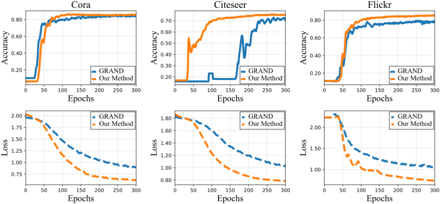
To further validate the performance gain of LSPAN, we plot the curves of testing accuracy and loss function for consistency learning with LSPAN and the GRAND method in Figure ??. We test on three datasets - CORA, CITESEER and FLICKR. We test on FLICKR because the LSPAN method is performed by augmenting feature matrix and the FLICKR dataset has a total number of 12,047 features, which shows the effectiveness of LSPAN on datasets with large feature dimensions. For all datasets, the MOP model is used as the backbone model. From the results, we observe that by adopting localized augmentation, our method converges in a more fast and stable manner, as well as achieving higher accuracies. This validates the good convergence property of consistency learning with LSPAN and verifies the benefit of our proposal.
5.3 Ablation Study
An ablation study is also conducted to verify the necessity of the introduced localized augmentation and examine whether it can be paired with other techniques. Specifically, we compare consistency learning with LSPAN over MOP to several of its ablated variants in Table 2. "w/o Localized AUG" means that we use random DropNode for augmentation. This is reasonable because LSPAN is also performed in a random manner. The drop is 2.1% which clearly illustrates the importance of proposal. Besides, "w/o Multi-Sampling" means we only perform augmentation once per epoch (namely S = 1) and "w/o Sharpening Trick" means we do not use the sharpening trick when calculating the distribution center (namely t = 1). These two variants respectively witness drops of 0.5% and 0.9%, which means multi-sampling and sharpening trick also help when paired with LSPAN. Overall, the promising performance of consistency learning with LSPAN is mainly contributed by the proposed localized augmentation, and it can be easily combined with commonly used techniques.
6 Conclusion
In this paper, we study the issue of exploring high-quality graph augmentation methods for graph consistency learning. We identify that existing augmentations are spectrally nonlocalized, where important graph spectrums are perturbed over the entire frequency range and can be largely changed. To enhance the preservation of graph information, we propose a simple but effective LSPAN method to conduct spectrally localized augmentation. LSPAN perturbs only a small concentrated part of graph spectrum, improves the preservation of spectrum structure and therefore benefits model prediction. Extensive empirical evaluation on real-world benchmarks shows that, by leveraging localized augmentation, graph consistency learning achieves considerable performance gains and always outperforms previous state-of-the-art methods.
Acknowledgments
This research was supported by the National Science Foundation of China (62306133, 62176118).
@inproceedings{ijcai2024p604,
  title     = {LSPAN: Spectrally Localized Augmentation for Graph Consistency Learning},
  author    = {Zhang, Heng-Kai and Zhang, Yi-Ge and Zhou, Zhi and Li, Yu-Feng},
  booktitle = {Proceedings of the Thirty-Third International Joint Conference on
               Artificial Intelligence, {IJCAI-24}},
  publisher = {International Joint Conferences on Artificial Intelligence Organization},
  editor    = {Kate Larson},
  pages     = {5462--5470},
  year      = {2024},
  month     = {8},
  note      = {Main Track},
  doi       = {10.24963/ijcai.2024/604},
  url       = {https://doi.org/10.24963/ijcai.2024/604},
}
TY - CPAPER TI - LSPAN: Spectrally Localized Augmentation for Graph Consistency Learning AU - Zhang, Heng-Kai AU - Zhang, Yi-Ge AU - Zhou, Zhi AU - Li, Yu-Feng T2 - Proceedings of the Thirty-Third International Joint Conference on Artificial Intelligence, IJCAI-24 PB - International Joint Conferences on Artificial Intelligence Organization PY - 2024 SP - 5462 EP - 5470 DO - 10.24963/ijcai.2024/604 UR - https://doi.org/10.24963/ijcai.2024/604 ER -Copied
Machine-readable versions of this paper, for tools and AI agents:





