
Geometry-Guided Conditional Adaptation for Surrogate Models of Large-Scale 3D PDEs on Arbitrary Geometries
Proceedings of the Thirty-Third International Joint Conference on Artificial Intelligence. Main Track. Pages 5790-5798.
https://doi.org/10.24963/ijcai.2024/640
Keywords
- Machine Learning: ML: Supervised Learning
- Multidisciplinary Topics and Applications: MTA: Physical sciences
- Computer Vision: CV: Transfer, low-shot, semi- and un- supervised learning
- Computer Vision: CV: 3D computer vision
Abstract
Deep learning surrogate models aim to accelerate the solving of partial differential equations (PDEs) and have achieved certain promising results. Although several main-stream models through neural operator learning have been applied to delve into PDEs on varying geometries, they were designed to map the complex geometry to a latent uniform grid, which is still challenging to learn by the networks with general architectures. In this work, we rethink the critical factors of PDE solutions and propose a novel model-agnostic framework, called 3D Geometry-Guided Conditional adaptation (3D-GeoCA), for solving PDEs on arbitrary 3D geometries. Starting with a 3D point cloud geometry encoder, 3D-GeoCA can extract the essential and robust representations of any kind of geometric shapes, which conditionally guides the adaptation of hidden features in the surrogate model. We conduct experiments on two public computational fluid dynamics datasets, the Shape-Net Car and Ahmed-Body dataset, using several surrogate models as the backbones with various point cloud geometry encoders to simulate corresponding large-scale Reynolds Average Navier-Stokes equations. Equipped with 3D-GeoCA, these backbone models can reduce the L-2 error by a large margin. Moreover, this 3D-GeoCA is model-agnostic so that it can be applied to any surrogate model.
- [Ahmed et al., 2019] S. R. Ahmed, G. Ramm, and G. Faitin. Some salient features of the time -averaged ground vehicle wake. Sae Paper, 840300, 2019.
- [Anandkumar et al., 2020] Anima Anandkumar, Kamyar Azizzadenesheli, Kaushik Bhattacharya, Nikola Kovachki, Zongyi Li, Burigede Liu, and Andrew Stuart. Neural op- erator: Graph kernel network for partial differential equa- tions. In ICLR 2020 Workshop on Integration of Deep Neu- ral Models and Differential Equations, 2020.
- [Belbute-Peres et al., 2020] Filipe De Avila Belbute-Peres, Thomas Economon, and Zico Kolter. Combining differ- entiable pde solvers and graph neural networks for fluid flow prediction. In international conference on machine learning, pages 2402-2411. PMLR, 2020.
- [Bonnet et al., 2022a] Florent Bonnet, Jocelyn Mazari, Paola Cinnella, and Patrick Gallinari. Airfrans: High fidelity computational fluid dynamics dataset for ap- proximating reynolds-averaged navier-stokes solutions. Advances in Neural Information Processing Systems, 35:23463-23478, 2022.
- [Bonnet et al., 2022b] Florent Bonnet, Jocelyn Ahmed Mazari, Thibaut Munzer, Pierre Yser, and Patrick Gal- linari. An extensible benchmarking graph-mesh dataset for studying steady-state incompressible navier-stokes equations. In ICLR 2022 Workshop on Geometrical and Topological Representation Learning, 2022.
- [Chang et al., 2015] Angel X Chang, Thomas Funkhouser, Leonidas Guibas, Pat Hanrahan, Qixing Huang, Zimo Li, Silvio Savarese, Manolis Savva, Shuran Song, Hao Su, et al. Shapenet: An information-rich 3d model repository. arXiv preprint arXiv:1512.03012, 2015.
- [Hamilton et al., 2017] Will Hamilton, Zhitao Ying, and Jure Leskovec. Inductive representation learning on large graphs. Advances in neural information processing sys- tems, 30, 2017.
- [Hughes, 2012] Thomas JR Hughes. The finite element method: linear static and dynamic finite element analysis. Courier Corporation, 2012.
- [Li et al., 2020a] Zongyi Li, Nikola Kovachki, Kamyar Az- izzadenesheli, Burigede Liu, Andrew Stuart, Kaushik Bhattacharya, and Anima Anandkumar. Multipole graph neural operator for parametric partial differential equa- tions. Advances in Neural Information Processing Sys- tems, 33:6755-6766, 2020.
- [Li et al., 2020b] Zongyi Li, Nikola Borislavov Kovachki, Kamyar Azizzadenesheli, Kaushik Bhattacharya, Andrew Stuart, Anima Anandkumar, et al. Fourier neural operator for parametric partial differential equations. In Interna- tional Conference on Learning Representations, 2020.
- [Li et al., 2022] Zongyi Li, Daniel Zhengyu Huang, Burigede Liu, and Anima Anandkumar. Fourier neural operator with learned deformations for pdes on general geometries. arXiv preprint arXiv:2207.05209, 2022.
- [Li et al., 2023a] Junnan Li, Dongxu Li, Silvio Savarese, and Steven Hoi. Blip-2: Bootstrapping language-image pre- training with frozen image encoders and large language models. arXiv preprint arXiv:2301.12597, 2023.
- [Li et al., 2023b] Zongyi Li, Nikola Borislavov Kovachki, Chris Choy, Boyi Li, Jean Kossaifi, Shourya Prakash Otta, Mohammad Amin Nabian, Maximilian Stadler, Chris- tian Hundt, Kamyar Azizzadenesheli, et al. Geometry- informed neural operator for large-scale 3d pdes. In Thirty-seventh Conference on Neural Information Pro- cessing Systems, 2023.
- [Mu et al., 2022] Norman Mu, Alexander Kirillov, David Wagner, and Saining Xie. Slip: Self-supervision meets language-image pre-training. In European Conference on Computer Vision, pages 529-544. Springer, 2022.
- [Pfaff et al., 2020] Tobias Pfaff, Meire Fortunato, Alvaro Sanchez-Gonzalez, and Peter W Battaglia. Learning mesh-based simulation with graph networks. arXiv preprint arXiv:2010.03409, 2020.
- [Qi et al., 2017] Charles Ruizhongtai Qi, Li Yi, Hao Su, and Leonidas J Guibas. Pointnet++: Deep hierarchical feature learning on point sets in a metric space. Advances in neu- ral information processing systems, 30, 2017.
- [Qian et al., 2022] Guocheng Qian, Yuchen Li, Houwen Peng, Jinjie Mai, Hasan Hammoud, Mohamed Elhoseiny, and Bernard Ghanem. Pointnext: Revisiting pointnet++ with improved training and scaling strategies. Advances in Neural Information Processing Systems, 35:23192-23204, 2022.
- [Raissi et al., 2019] Maziar Raissi, Paris Perdikaris, and George E Karniadakis. Physics-informed neural networks: A deep learning framework for solving forward and in- verse problems involving nonlinear partial differential equations. Journal of Computational physics, 378:686- 707, 2019.
- [Ronneberger et al., 2015] Olaf Ronneberger, Philipp Fis- cher, and Thomas Brox. U-net: Convolutional networks for biomedical image segmentation. In Medical Image Computing and Computer-Assisted Intervention-MICCAI 2015: 18th International Conference, Munich, Germany, October 5-9, 2015, Proceedings, Part III 18, pages 234- 241. Springer, 2015.
- [Smith and Topin, 2019] Leslie N Smith and Nicholay Topin. Super-convergence: Very fast training of neural networks using large learning rates. In Artificial intelli- gence and machine learning for multi-domain operations applications, volume 11006, pages 369-386. SPIE, 2019.
- [Strikwerda, 2004] John C Strikwerda. Finite difference schemes and partial differential equations. SIAM, 2004.
- [Tran et al., 2022] Alasdair Tran, Alexander Mathews, Lex- ing Xie, and Cheng Soon Ong. Factorized fourier neural operators. In The Eleventh International Conference on Learning Representations, 2022.
- [Umetani and Bickel, 2018] Nobuyuki Umetani and Bernd Bickel. Learning three-dimensional flow for interactive aerodynamic design. ACM Transactions on Graphics (TOG), 37(4):1-10, 2018.
- [Veličković et al., 2018] Petar Veličković, Guillem Cucurull, Arantxa Casanova, Adriana Romero, Pietro Liò, and Yoshua Bengio. Graph attention networks. In Interna- tional Conference on Learning Representations, 2018.
- [Xue et al., 2023a] Le Xue, Mingfei Gao, Chen Xing, Roberto Martín-Martín, Jiajun Wu, Caiming Xiong, Ran Xu, Juan Carlos Niebles, and Silvio Savarese. Ulip: Learning a unified representation of language, images, and point clouds for 3d understanding. In Proceedings of the IEEE/CVF Conference on Computer Vision and Pattern Recognition, pages 1179-1189, 2023.
- [Xue et al., 2023b] Le Xue, Ning Yu, Shu Zhang, Junnan Li, Roberto Martín-Martín, Jiajun Wu, Caiming Xiong, Ran Xu, Juan Carlos Niebles, and Silvio Savarese. Ulip-2: To- wards scalable multimodal pre-training for 3d understand- ing. arXiv preprint arXiv:2305.08275, 2023.
- [Yu et al., 2022] Xumin Yu, Lulu Tang, Yongming Rao, Tiejun Huang, Jie Zhou, and Jiwen Lu. Point-bert: Pre- training 3d point cloud transformers with masked point modeling. In Proceedings of the IEEE/CVF Conference on Computer Vision and Pattern Recognition, pages 19313- 19322, 2022.
References were extracted automatically from the PDF and may contain errors.
Full text extracted automatically from the PDF; figures, tables and equations may differ. The PDF is the version of record.
1 Introduction
Partial differential equation (PDE) is a powerful model to describe various physical phenomena and help us to understand this world to a large extent. However, most PDEs do not have closed-form solutions, which leads to a resort to numerical methods for solving them. Actually, various approaches have been proposed, including finite difference [Strikwerda, 2004] and finite element methods [Hughes, 2012], whereas these methods usually have high computational costs, which are unendurable in many real-time settings. As a data-driven method, the deep learning surrogate model can learn from numerical solutions to a family of PDEs and generalize well to the unseen equations via forward propagation within a second, which is much faster than traditional numerical solvers, exhibiting a promising future.
While traditional numerical solvers usually simulate PDEs on irregular mesh grids with various geometries, it is possible to reformulate the input data into uniform grids and employ convolution-based architectures such as U-Net [Ronneberger et al., 2015] to train surrogate models. However, this approach may not be as efficient and can introduce additional interpolation error [Li et al., 2022]. To address these challenges, several researchers have turned to Graph Neural Networks (GNNs) as the backbone of surrogate models [BelbutePeres et al., 2020; Pfaff et al., 2020]. Furthermore, Bonnet el al. [2022b; 2022a] introduced certain benchmarking graphmesh datasets using graph or point cloud input data. In their work, they employed Point Cloud Networks to solve the 2D steady-state incompressible Navier-Stokes equations.
Another stream of research focuses on the Neural Operator Learning paradigm, which aims to learn a mapping between infinite-dimensional function spaces. Li et al. [2020b] made theoretical analyses and proposed a novel iterative architecture utilizing the kernel integral operator. When the input type is uniform grids, Fast Fourier Transform (FFT) is used to implement the kernel integral operator. This operator, known as FNO [Li et al., 2020b], transforms features in both the physical and spectral domains. To handle irregular grid inputs, Anandkumar et al. [2020] introduced the Graph Neural Operator (GNO), where the kernel integral operator is formulated as message passing on a radius graph. These two neural operators have been widely adopted and have spawned numerous improved methods capable of solving PDEs with varying geometries, including Multipole GNO (MGNO) [Li et al., 2020a], Geo-FNO [Li et al., 2022], and GeometryInformed Neural Operator (GINO) [Li et al., 2023b].
Although the above works have achieved remarkable progress in solving 2D equations, many real-world applications face the problem of 3D PDEs on varying geometries, ranging from industrial and engineering design to realtime physics simulation engines in games and virtual reality. When it comes to solving more complex 3D problems, the mentioned state-of-the-art approaches have severe limitations as follows:
Inefficient Representation for 3D Inputs: Most existing methods treat all positions within the field-both boundary and interior points-equally, feeding all grids into the model in a coarse manner [Bonnet et al., 2022a; Bonnet et al., 2022b]. However, such an approach can hinder the learning of geometry features crucial for PDE solving, as the boundary points carry more information than the other points to represent a geometry. In this sense, current methods inefficiently represent the input field, which becomes more serious as the input dimension increases to 3D.
Poor Generalization on Limited Training Samples: Another limitation lies in the scarcity of training data. Generating a dataset for the deep learning surrogate model is computationally intensive and time-consuming. For instance, creating a Computational Fluid Dynamics (CFD) Ahmed-Body dataset with 551 samples required Li et al. [2023b] to conduct large-scale 3D simulations on 2 NVIDIA V100 GPUs and 16 CPU cores, each simulation of a sample lasting 7 to 19 hours. The limited number of training samples further complicates learning geometry features that can be generalized to unknown shapes, thus compromising the model's generalization capabilities.
To overcome the above challenges, we propose a brand new model-agnostic framework, 3D Geometry-Guided Conditional Adaptation (3D-GeoCA). Based on a general deep learning architecture, 3D-GeoCA adopts a novel method which conditionally guides the adaptation of hidden features with latent geometry representations. The involved point cloud geometry encoder has low computational cost since it computes only on the boundary points that occupy a very small portion of the input field. Regarding the problem of data scarcity, we apply the weight transfer by utilizing some pre-trained point cloud models. Equipped with 3D-GeoCA, the backbone model becomes more geometry-aware and generalizes better on small-sample 3D PDE datasets. The main contributions of our paper are as follows:
- We propose a novel framework, called 3D GeometryGuided Conditional adaptation (3D-GeoCA), for solving large-scale 3D PDEs on arbitrary geometries. 3DGeoCA originally introduces a point cloud geometry encoder to encode the boundary of the problem domain, and conditionally guides the adaptation of hidden features in the backbone model with geometry information. Experimental results on two 3D PDE datasets demonstrate that our framework provides generalizable geometry features beneficial to the backbone surrogate model, which is lacking in the other approaches.
- Our 3D-GeoCA is model-agnostic and orthogonal to various deep learning based 3D PDE frameworks, including MLP, GNN, GNO and so on.
- To the best of our knowledge, our framework unprecedentedly introduces 3D understanding pre-training to the deep surrogate model for PDEs to alleviate the shortage of training samples, bridging the relationship between these two fields.
2 Problem Setting and Preliminaries
Problem setting. We consider a family of PDEs with varying domains of the following general form:
where La is a differential operator describing the governing equation, being parameterized by a; f and g respectively denote corresponding initial and boundary conditions; and Dω is the problem domain, being parameterized by some latent parameters ω ∈ Ω.
In practical applications, we ideally assume that there exists a map F : (a, f, g,Dω) ↦→ u which gives the solution of equations 1. Here, we mainly consider the steady-state equations, where u is independent of the time t, equations 1 convert to Lau(x) = 0 and the solution map simplifies to F : (a, g,Dω) ↦→ u, from which we clearly aware that the boundary of the domain, ∂Dω, is a decisive factor to the solution u.
However, learning the geometry of ∂Dω from a small dataset is rather challenging, especially for 3D cases. We believe that this is one of the bottlenecks current studies have to confront. Considering that the boundary ∂Dω can be discretized to the point cloud data, we introduce a point cloud encoder to enrich the learning of geometries. Moreover, a state-of-the-art 3D understanding pre-training framework, ULIP-2 [Xue et al., 2023b], is adopted to strengthen our encoder. By using point cloud models pre-trained on large-scale 3D object datasets, we can learn better geometry features to solve this dilemma.
Preliminaries: ULIP-2. Deriving from the Unified Representation of Language, Images, and Point Clouds (ULIP) framework proposed by Xue et al. [2023a], ULIP-2 is a tri-modal pre-training framework, which leverages a pseudo self-supervised contrastive learning approach to align features across: (i) 3D shapes, (ii) their rendered 2D image counterparts, and (iii) the language descriptions of 2D images of all views. Among them, language descriptions of 2D images come from BLIP-2 [Li et al., 2023a], a large multimodal model. In ULIP-2, a fixed and pre-aligned languagevision model, SLIP [Mu et al., 2022], is used to extract text and image features, after which the authors train point cloud encoders under the guidance of 3D-to-image and 3D-to-text contrastive alignment losses. ULIP-2 yields significant improvements on downstream zero-shot and standard classification tasks, showing a powerful capability for 3D representation learning.
3 3DGeometry-Guided Conditional Adaptation
In this section, we present our framework, 3D-GeoCA, in detail. The key insight of 3D-GeoCA is the emphasis on the geometries inherent in various PDE problem domains. To capture these geometries, we introduce a specialized geometry encoder. Furthermore, we propose an adaptor that seamlessly integrates with existing surrogate backbone models. Figure 1 provides an overview of the main architecture of 3D-GeoCA. As a model-agnostic framework, 3D-GeoCA comprises three primary components: (i) a point cloud geometry encoder (blue), (ii) an arbitrary backbone model (yellow), and (iii) geometry-guided conditional adaptors (red). The point cloud encoder solely relies on the boundary of the problem domain to extract its geometry features. Conversely, the backbone model considers the entire problem domain, along with the signed distance function (SDF) and normal vector features of each grid. Finally, a crucial part of our framework is the design of several geometry-guided conditional adaptors, which facilitate the fusion of geometry features with the hidden features of the backbone surrogate model.
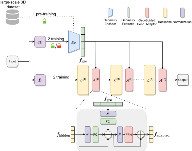
Point cloud geometry encoder. As per previous discussions in section 2, one of the bottlenecks of current work is the under-exploited geometry features of various problem domains. To overcome this difficulty, we propose a point cloud encoder EP specialized to extract features of different geometries, whose input is a 3D point cloud P = {x∂D 1 , x∂D 2 , · · · , x∂D n } ⊂ ∂D discretized from the boundary of the problem domain D.
Compared to the whole problem domain D, the point cloud P ⊂ ∂D usually contains a tiny part of the input grids (especially for 3D settings), thus leading to a relatively low computational cost. Current work usually under-emphasizes grids in P ⊂ ∂D and coarsely feeds all grids with simple hand-crafted features (such as SDF) into their model [Bonnet et al., 2022b; Bonnet et al., 2022a]. However, this may lead to a loss in the learning of geometries, as the small portion of grids at the boundary contains most underlying geometry information of the problem domain D.
To improve our encoder EP , we employ a state-of-the-art 3D understanding pre-training framework, ULIP-2, to pretrain it on large-scale 3D object datasets. Once the encoder is pre-trained, the parameters of EP can either be fine-tuned or fixed. In the latter case, we can further reduce the number of trainable parameters and shorten the training process without seriously harming the effectiveness of our framework. See section 4.4 for experimental details.
Backbone models. As a model-agnostic framework, 3DGeoCA is compatible with arbitrary backbone models, ranging from the basic multi-layer perceptron (MLP) to the GNO that follows the popular neural operator learning paradigm. In our work, the backbone model aims to solve PDEs in the problem domain D and its boundary ∂D. It takes either the point cloud data V or graph data G = (V, E) as input, where the vertex set V = {x ¯D1 , x ¯D2 , · · · , x ¯DN } ⊂ ¯D = D∪ ∂D contains all grids of interest. We also compute the SDF feature and normal vector to ∂D for each vertex as a part of feature engineering. For the graph-based backbone model, the edge set E can be constructed according to the corresponding meshes or the radius graph with a maximum number of neighbors [Bonnet et al., 2022b]. In this way, we can prevent the degree of each vertex from being too large and reduce the computation complexity.
Geometry-guided conditional adaptor. We propose a geometry-guided conditional adaptor, which enables the adaptation of hidden features according to various geometries. At first, the adaptor conducts a feature fusion between hidden features in the backbone model and geometry features extracted by the point cloud encoder. Then, a feed-forward network processes the fused features to add non-linearity. Skip connections, normalization layers, and dropout layers are also added to our adaptor.
Denote f (l) hidden as the hidden features output by the l-th layer of the backbone model (l = 1, 2, · · · , L), and fgeo = EP (P) as the geometry features extracted by the point cloud encoder EP . Formally, each adaptor can be formulated as follows:
and
where W (l) hidden andW (l) geo are learnable parameters and norm(·) represents L-2 layer normalization. Equation 2 describes the process of feature fusion, by which we yield the fused feature f (l) fused of the l-th layer. In equation 3, f (l) fused are input into a feed-forward network to acquire adapted features f (l) adapted of the l-th layer.
Finally, the adapted features f (l) adapted are fed into the (l + 1)-th layer of the backbone model to get the hidden features f (l+1) hidden of the (l +1)-th layer.
Although our adaptor introduces additional structures to the backbone model, it requires only O(h∗(h+hgeo)) parameters, where h is the hidden size of the backbone model and hgeo is the dimension of geometry features. Thus, our adaptor brings relatively low computational cost and inference latency once the backbone is a large model. As an example, an original 3D FNO layer with hidden size h requires O(h2M 3 ) parameters, where M is the number of top Fourier modes being kept and usually be a large number, ranging from O(101 ) to O(102 ).
4 Experiments
To empirically validate our findings, we conduct experiments on the public Shape-Net Car CFD dataset generated by Umetani and Bickel [2018] and the Ahmed-Body dataset generated by Li et al. [2023b]. Several previous works have explored these datasets [Umetani and Bickel, 2018; Li et al., 2023b], while Umetani and Bickel [2018] adopted the Gaussian process regression approach that falls outside the category of deep learning. Li et al. [2023b] also proposed the powerful GINO model for 3D PDEs with varying geometries, whereas their goal was to predict the pressure field at the boundary of the problem domain, namely ∂D. In contrast, we intend to simultaneously simulate plural physical properties (including both pressure and velocity) at all grids of interest in ¯D = D ∪ ∂D. We trail multiple architectures of the point cloud geometry encoder and the backbone model, and all experiments can run on a single NVIDIA RTX A6000 GPU.
4.1 Shape-Net Car CFDDataset
The Shape-Net Car CFD Dataset was generated to study how fluid flows around various 3D objects [Umetani and Bickel,
2018]. In that work, different object shapes of cars from the "car" category of ShapeNet [Chang et al., 2015] were prepared, with their side mirrors, spoilers, and tries manually removed. The dataset contains 889 samples, each of which is a simulation result of a finite element solver. During the simulation, time-averaged fluid pressure on the surface and velocity field around the car was computed by solving the large-scale Reynolds Average Navier-Stokes equations with the k-ϵ turbulence model and SUPG stabilization. All the simulations ran with a fixed inlet velocity of 72 km/h and a Reynolds number of 5 × 10⁶ .
The dataset has already been randomly divided into nine folds. We take the first fold as our testing set, while the rest of the data consists of the training set. In each sample, the simulation result is discretized to 32k mesh grids, while the car surface counts merely 3.7k, implying that our backbone model and point cloud geometry encoder take 32k and 3.7k grids as input, respectively.
4.2 Ahmed-Body Dataset
The Ahmed-Body Dataset [Li et al., 2023b] contains 551 industry-level vehicle aerodynamics simulation samples based on Ahmed-body shapes [Ahmed et al., 2019], 500 for training and the others 51 for testing. All the simulations were conducted using the SST k-ω turbulence model, with the inlet velocity ranging from 10m/s to 70m/s. For each sample, the computational mesh consisted of 7.2 million grids overall, with 100k of those points at the surface.
Currently, merely the pressure data at the surface are available, therefore we use our framework to predict them.
4.3 Experimental Settings
Backbone models. Multiple architectures of the backbone model and the point cloud geometry encoder are employed to demonstrate the effectiveness of our framework. Since 3DGeoCA is a groundbreaking framework that correlates PDEs with the field of 3D understanding, we start with the simple MLP as our backbone model. Several classical GNNs, such as GraphSAGE [Hamilton et al., 2017] and Graph Attention Network (GAT) [Veliˇckovi´c et al., 2018] are also attempted in later. We also explore the application of 3D-GeoCA in the popular neural operator learning paradigm, where we consider GNO due to its ability to deal with irregular grid input directly. For Ahmed-Body dataset, since each sample consists of 100k data points, it is challenging for some graphbased models to scale up, so we only attempt to train two relative simple backbones, MLP and GraphSAGE.
Point cloud geometry encoders. As for the point cloud geometry encoder, we trial with two state-of-the-art point cloud architectures, Point-BERT [Yu et al., 2022] and PointNeXt [Qian et al., 2022]. Point-BERT adopts transformerbased architecture, while PointNeXt is a lightweight backbone based on PointNet++ [Qi et al., 2017] with improved training and scaling strategies. Both point cloud models are pre-trained with the ULIP-2 framework on the Objaverse Triplets dataset [Xue et al., 2023b] to promote their capabilities to learn 3D geometry representations.
Training schemes. We normalize all inputs and outputs for data pre-processing. Since we target to predict the pressure and velocity by one forward propagation, we use the following weighted MSE loss to train models:
| Geo. Encoder Backbone | MLP | GraphSAGE | GAT | GNO | ||||
|---|---|---|---|---|---|---|---|---|
| None | 8.044 | 0.556 | 6.590 | 0.523 | 6.128 | 0.525 | 5.120 | 0.434 |
| 3D-GeoCAw/ PointNeXt (frozen) | 6.705 | 0.375 | 5.618 | 0.363 | 5.510 | 0.355 | 4.970 | 0.386 |
| (-17%) | (-33%) | (-15%) | (-31%) | (-10%) | (-32%) | (-3%) | (-11%) | |
| 3D-GeoCAw/ Point-BERT (frozen) | 6.456 | 0.368 | 5.630 | 0.349 | 5.629 | 0.346 | 4.991 | 0.365 |
| (-20%) | (-34%) | (-15%) | (-33%) | (-8%) | (-34%) | (-3%) | (-16%) | |
| 3D-GeoCAw/ Point-BERT (fine-tuned) | 5.916 | 0.352 | 5.569 | 0.349 | 5.438 | 0.339 | 4.906 | 0.356 |
| (-26%) | (-37%) | (-15%) | (-33%) | (-11%) | (-35%) | (-4%) | (-18%) | |
where N denotes the number of training samples. v(i) j and p(i) j represent velocity and pressure of the i-th sample at the jth grid, respectively. n(i) denotes the number of input grids in the i-th sample, and m(i) = ∑n(i) j=1 I(x(i) j ∈ ∂D) is the number of boundary grids in the i-th sample. The hyper-parameter λ balances the weight of the error between velocity and pressure, taking the default value of 0.5.
We train our models with Adam optimizer and one-cycle learning rate scheduler [Smith and Topin, 2019]. The batch size B = 11 , and the maximum and minimum learning rates are 1×10⁻³ and 1×10⁻⁶ , respectively. For the GNO backbone, the hidden size h = 32, and we train models for 200 epochs to save GPU memories and training times. Models of other backbones are trained for 400 epochs with the hidden size h = 64. For Ahmed-Body dataset, all models are trained for 100 epochs, the same experimental settings as Li et al. [2023b], for a fair comparison. For more implementation details, please see appendix A.1.
Evaluation metrics. Following previous work [Anandkumar et al., 2020; Li et al., 2020b; Li et al., 2023b; Tran et al., 2022], we introduce L-2 error and relative L-2 error to evaluate our models, which are defined as
1B = 1 implies that we train the model on a batch of 32k graph nodes for Shape-Net Car dataset and 100k for Ahmed-Body dataset, respectively.
and
where u represents the physical property of interest.
4.4 Results and Comparisons
The effectiveness of 3D-GeoCA. Table 1 illustrates test L-2 errors of multiple backbone models with various point cloud geometry encoders on the Shape-Net Car dataset. Since PointNeXt requires a training batch size greater than 1 to apply batch normalization, we keep its parameters frozen and do not fine-tune them. From table 1, we notice that 3D-GeoCA universally promotes all backbone models, reducing their L2 errors by a large margin. For instance, with the trainable Point-BERT geometry encoder, MLP yields a marked descent in L-2 errors by 26% and 37% for pressure and velocity, respectively. The GNO 2 , which follows the paradigm of operator learning, also benefits from our 3D-GeoCA framework, with its L-2 errors decreasing by 4% for pressure and 18% for velocity. By introducing a specialized geometry encoder, we take full advantage of the rich geometry information, and our adaptors enable backbone models to become more geometryaware to generalize to unknown shapes.
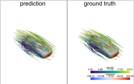
At the inference stage, our proposed 3D-GeoCA with Point-BERT (fine-tuned) encoder merely takes 0.066 second for each sample in the Shape-Net Car dataset, which is much faster than traditional numerical solvers. As a comparison, in their efforts to generate that dataset, Umetani and Bickel [2018] spent about 50 minutes per sample to run the simulations using traditional solvers. Figure 2 visualizes a ground truth and prediction generated by the GNO backbone with the Point-BRET (fine-tuned) encoder. For more visualization examples, please see appendix A.5.
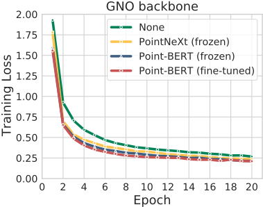
Moreover, 3D-GeoCA accelerates the convergence of the backbone model as well. Figure 3 exhibits the training loss of the GNO backbone with different geometry encoders for the beginning 20 epochs. The training loss of the GNO baseline decreases slowly, while the other three models equipped with 3D-GeoCA show higher convergence rates.
2 We use a variant of GNO which utilizes hexahedral meshes generated by Umetani and Bickel [2018] to construct graphs. For original GNO, we also conduct experiments, see appendix A.2 for details.
| Geo. Encoder Backbone | MLP | GraphSAGE | GINO (enc-dec) | GINO (dec) | ||
|---|---|---|---|---|---|---|
| None | 41.417 | 11.86% | 44.937 | 12.87% | - 8.31% 3 | - 9.01% 3 |
| 3D-GeoCAw/ PointNeXt (frozen) | 28.579 | 7.76% | 30.662 | 8.73% | - - | - - |
| 3D-GeoCAw/ Point-BERT (frozen) | 29.946 | 8.12% | 31.282 | 8.55% | - - | - - |
| 3D-GeoCAw/ Point-BERT (fine-tuned) | 28.056 | 7.56% | 29.857 | 8.26% | - - | - - |
We also conduct experiments on the Ahmed-Body dataset, and table 2 exhibits corresponding results. The introduction of 3D-GeoCA also yields consistent improvement to the backbone models across different backbone models and geometry encoders. Among them, the MLP backbone with Point-BERT (fine-tuned) encoder gains the lowest relative L2 error of 7.56%.
3 The results are from [Li et al., 2023b].
Discussions on different geometry encoders. Surprisingly, we observe that once pre-trained, even though the geometry encoder keeps frozen during training, it still extracts useful geometry information that can guide the adaptation in the backbone model. As shown in table 1 and 2, the fixed PointNeXt and Point-BERT features pre-trained by ULIP2 still perform well in the 3D-GeoCA framework and lead to competitive results compared to the fine-tuned features. This finding is of great significance, implying that under our 3D-GeoCA framework, 3D understanding pre-training techniques may directly enhance the performance of PDEs surrogate models. Moreover, once the geometry encoder is frozen, we can pre-calculate geometry features and reduce the number of learnable parameters during training, further shortening the training process. Our GNO backbone with pretrained features requires merely 0.6 million trainable parameters while reaching competitive low L-2 and relative L-2 errors.
The impact of various backbones. As a novel framework that unprecedentedly correlates PDEs with the field of 3D understanding, we start with the simple MLP as our backbone model. Conceptually, according to the discussion in section 2, in steady-state equations with fixed parameters a and boundary conditions g, the physical property u at (x, y, z) is merely decided by the geometry of problem domain D and its coordinate (x, y, z). This explains why MLP backbone performs competitive well compared to GraphSAGE in the Ahmed-Body dataset, as shown in table 2. Another factor we need to point out is that we construct relatively less number of edges for each sample in this large dataset to save computational costs, which may lead a insufficient training for GNN. However, table 1 indicates that on the Shape-Net Car dataset, the simple MLP gains relatively large L-2 errors compared to other backbones. We conjecture that this may be because the ground truth u of this dataset is a smooth function, and adjacent data points may share similar features. With the introduction of graph input structure, GNNs can learn better features from adjacent nodes via the message-passing mechanism. Consistent with our analysis, GraphSAGE and GAT perform better than MLP on this dataset. Differing the above backbones, GNO aims to learn operators that map between function spaces via the kernel integration mechanism and shows an advantage in predicting pressure fields in our experiments.
| Geo. Encoder Backbone | MLP | GraphSAGE | GAT | GNO | ||||
|---|---|---|---|---|---|---|---|---|
| None (bs=1) | 8.044 | 0.556 | 6.590 | 0.523 | 6.128 | 0.525 | 5.120 | 0.434 |
| None (bs=2) | 9.976 | 0.688 | 7.470 | 0.611 | 6.957 | 0.622 | 5.872 | 0.517 |
| 3D-GeoCAw/ PointNeXt (frozen, bs=1) | 6.705 | 0.375 | 5.618 | 0.363 | 5.510 | 0.355 | 4.970 | 0.386 |
| 3D-GeoCAw/ PointNeXt (frozen, bs=2) | 8.758 | 0.546 | 6.293 | 0.467 | 6.273 | 0.471 | 5.581 | 0.479 |
| 3D-GeoCAw/ Point-BERT (frozen, bs=1) | 6.456 | 0.368 | 5.630 | 0.349 | 5.629 | 0.346 | 4.991 | 0.365 |
| 3D-GeoCAw/ Point-BERT (frozen, bs=2) | 7.796 | 0.437 | 5.909 | 0.411 | 5.922 | 0.399 | 5.329 | 0.411 |
| 3D-GeoCAw/ Point-BERT (fine-tuned, bs=1) | 5.916 | 0.352 | 5.569 | 0.349 | 5.438 | 0.339 | 4.906 | 0.356 |
| 3D-GeoCAw/ Point-BERT (fine-tuned, bs=2) | 6.689 | 0.423 | 5.571 | 0.360 | 5.454 | 0.351 | 4.957 | 0.374 |
Comparisons with other works. For the Shape-Net Car dataset, GNO with the trainable Point-BERT encoder achieves the lowest test loss in our experiments, with the L-2 error (relative L-2 error) of pressure and velocity of 4.906 (7.79%) and 0.356 (3.19%), respectively. As some reference values, the Gaussian Process Regression approach proposed by Umetani and Bickel [2018] reached a nine-fold mean L-2 error of 8.1 for pressure and 0.48 for velocity. The previous work GINO [Li et al., 2023b] reported a relative L-2 error of pressure of 7.19% for GINO (decoder) and 9.47% for GINO (encoder-decoder). The relative L-2 error of GINO (decoder) is lower than that of our current experiments, though we should mention that their work has different training schemes and train-test split from ours. Another factor is that the GINO adopts a complex GNO-FNO architecture, while we have merely explored GNO as our backbone model. Moreover, the GINO can only simulate the pressure field at the surface of each car (3.7k grids). As the opposite, we train our models to simultaneously predict the velocity field around the car (32k grids) as well. For Ahmed-Body dataset, the MLP backbone equipped with Point-BERT (fine-tuned) encoder reaches the state-of-the-art lowest relative L2 error of 7.56%, outperforming GINO with either encoder-decoder or decoder-only architectures.
4.5 Ablation Studies
The selection of batch size. During experiments, we find that the training batch size is the most critical hyper-parameter that impacts the quality of training. Table 3 shows the test L2 errors under different batch sizes 4 , from which we observe that using a larger batch size during training brings a universal negative influence on our models, especially for simple architectures, such as models with MLP backbone and models with no geometry encoder. When the model structure becomes complex, there is relatively less increase in test L-2 error. Although it is more obvious to validate the effectiveness of our 3D-GeoCA framework when the batch size B = 2, we set B = 1 in our experiments to ensure that every model obtains the best results.
4 We also fine-tune PointNeXt under B = 2, see appendix A.3
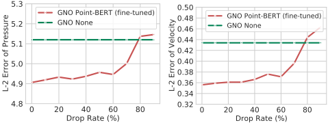
The robustness of geometry encoders. We further demonstrate the robustness of our fine-tuned geometry encoder by randomly dropping its input data points in the inference time. Figure 4 depicts how L-2 errors varied with the rate of dropping increases. Surprisingly, even if we drop each data point with a high probability of 60%, our encoder still extracts essential geometry features that can guide the adaptation of hidden features in the backbone model, demonstrating its strong robustness.
5 Conclusion
Learning the solution of 3D PDEs with varying geometries is challenging due to the complexity of 3D shapes and insufficient training samples. By introducing a specialized point cloud geometry encoder, our proposed 3D-GeoCA framework learns the essential and robust geometry features that can guide the adaptation of hidden features in the backbone model. 3D understanding pre-training further enhances our framework. The experimental results demonstrate that several backbones can reduce the L-2 error by a large margin as they are equipped with 3D-GeoCA. So far, our way of conditional adaptation remains simple and effective, but may not be optimal. For future work, we are interested in exploring other effective and efficient structures for our adaptor. Moreover, we expect our framework to be compatible with the backbones of broader fields, such as FNO and Physics-Informed Neural Network (PINN) [Raissi et al., 2019].
Acknowledgements
This work was supported by the Natural Science Foundation of China under grant 62071171 and the high-performance computing platform of Peking University.
Contribution Statement
Jingyang Deng conceived the methodology, designed and conducted experiments, and drafted the manuscript. Xingjian Li, as the co-first author, contributed to the research conception, delineated the research direction, and also participated in drafting the manuscript. Haoyi Xiong supervised the research planning and execution, provided constructive suggestions, and critically reviewed the manuscript. Xiaoguang Hu provided valuable insights and expertise during the research progress. Jinwen Ma, as the corresponding author, administered the research project, provided the funding and computing resources, supervised the research process and revised the manuscript.
@inproceedings{ijcai2024p640,
  title     = {Geometry-Guided Conditional Adaptation for Surrogate Models of Large-Scale 3D PDEs on Arbitrary Geometries},
  author    = {Deng, Jingyang and Li, Xingjian and Xiong, Haoyi and Hu, Xiaoguang and Ma, Jinwen},
  booktitle = {Proceedings of the Thirty-Third International Joint Conference on
               Artificial Intelligence, {IJCAI-24}},
  publisher = {International Joint Conferences on Artificial Intelligence Organization},
  editor    = {Kate Larson},
  pages     = {5790--5798},
  year      = {2024},
  month     = {8},
  note      = {Main Track},
  doi       = {10.24963/ijcai.2024/640},
  url       = {https://doi.org/10.24963/ijcai.2024/640},
}
TY - CPAPER TI - Geometry-Guided Conditional Adaptation for Surrogate Models of Large-Scale 3D PDEs on Arbitrary Geometries AU - Deng, Jingyang AU - Li, Xingjian AU - Xiong, Haoyi AU - Hu, Xiaoguang AU - Ma, Jinwen T2 - Proceedings of the Thirty-Third International Joint Conference on Artificial Intelligence, IJCAI-24 PB - International Joint Conferences on Artificial Intelligence Organization PY - 2024 SP - 5790 EP - 5798 DO - 10.24963/ijcai.2024/640 UR - https://doi.org/10.24963/ijcai.2024/640 ER -Copied
Machine-readable versions of this paper, for tools and AI agents:





