
Linear-Time Optimal Deadlock Detection for Efficient Scheduling in Multi-Track Railway Networks
Proceedings of the Thirty-Third International Joint Conference on Artificial Intelligence. Main Track. Pages 5799-5807.
https://doi.org/10.24963/ijcai.2024/641
Keywords
- Multidisciplinary Topics and Applications: MTA: Transportation
- Planning and Scheduling: PS: Applications
- Planning and Scheduling: PS: Markov decisions processes
- Planning and Scheduling: PS: Scheduling
Abstract
The railway scheduling problem requires the computation of an operable timetable that satisfies constraints involving railway infrastructure and resource occupancy times, while minimising average delay over a set of events. Since this problem is computationally hard, practical solutions typically roll out feasible (but suboptimal) schedules one step at a time, by choosing which train to move next in every step. The choices made by such algorithms are necessarily myopic, and incur the risk of driving the system to a deadlock. To escape deadlocks, the predominant approach is to stay away from states flagged as potentially unsafe by some fast-to-compute rule R. While many choices of R guarantee deadlock avoidance, they are suboptimal in the sense of also flagging some safe states as unsafe. In this paper, we revisit the literature on process scheduling and describe a rule R0 that is (i) necessary and sufficient for deadlock detection when the network has at least two tracks in each resource (station / track section), (ii) computable in linear time, and (iii) yields lower delays when combined with existing scheduling algorithms on both synthetic and real data sets from Indian Railways.
- [Agarwal, 2022] Keshav Agarwal. Real-time railway scheduling. Master's thesis, Indian Institute of Technol- ogy Bombay, 2022.
- [Araki et al., 1977] Toshiro Araki, Yuji Sugiyama, Tadao Kasami, and Jun Okui. Complexity of the deadlock avoid- ance problem. In 2nd IBM Symp. on Mathematical Foun- dations of Computer Science, pages 229-257, 1977.
- [Cai and Goh, 1994] X Cai and C Goh. A fast heuristic for the train scheduling problem. Computers & Op. Res., 21(5):499-510, 1994.
- [Chen et al., 2015] L Chen, C Roberts, F Schmid, and E Stewart. Modeling and solving real-time train reschedul- ing problems in railway bottleneck sections. IEEE Trans. on Intelligent Transportation Systems, 16(4):1896-1904, 2015.
- [Cocco and Monasson, 2001] Simona Cocco and Rémi Monasson. Trajectories in phase diagrams, growth processes, and computational complexity: How search algorithms solve the 3-satisfiability problem. Physical review letters, 86(8):1654, 2001.
- [Fanti et al., 1997] Maria Pia Fanti, Bruno Maione, Saverio Mascolo, and A Turchiano. Event-based feedback con- trol for deadlock avoidance in flexible production sys- tems. IEEE Transactions on Robotics and Automation, 13(3):347-363, 1997.
- [Gold, 1978] E Mark Gold. Deadlock prediction: Easy and difficult cases. SIAM Journal on Computing, 7(3):320- 336, 1978.
- [Goverde, 2010] Rob MP Goverde. A delay propaga- tion algorithm for large-scale railway traffic networks. Transportation Research Part C: Emerging Technologies, 18(3):269-287, 2010.
- [Higgins et al., 1996] A Higgins, E Kozan, and L Ferreira. Optimal scheduling of trains on a single line track. Trans- portation Research Part B, 30(2):147-161, 1996.
- [Higgins et al., 1997] A Higgins, E Kozan, and L Ferreira. Heuristic techniques for single line train scheduling. Jour- nal of Heuristics, 3(1):43-62, 1997.
- [Khadilkar, 2017a] Harshad Khadilkar. Data-enabled stochastic modeling for evaluating schedule robust- ness of railway networks. Transportation Science, 51(4):1161-1176, 2017.
- [Khadilkar, 2017b] Harshad Khadilkar. Scheduling of vehi- cle movement in resource-constrained transportation net- works using a capacity-aware heuristic. In 2017 Ameri- can Control Conference (ACC), pages 5617-5622. IEEE, 2017.
- [Khadilkar, 2018] Harshad Khadilkar. A scalable reinforce- ment learning algorithm for scheduling railway lines. IEEE Transactions on Intelligent Transportation Systems, 20(2):727-736, 2018.
- [Liu and Kozan, 2009] S Liu and E Kozan. Scheduling trains as a blocking parallel-machine job shop scheduling prob- lem. Computers & Operations Research, 36(10):2840- 2852, 2009.
- [Lovett et al., 2015] Alexander H Lovett, C Tyler Dick, and Christopher PL Barkan. Determining freight train delay costs on railroad lines in north america. Proceedings of Rail Tokyo, 2015.
- [Mackenzie, 2010] S. Mackenzie. Train scheduling on long haul railway corridors. PhD thesis, University of South Australia, 2010.
- [Manne, 1960] Alan S Manne. On the job-shop scheduling problem. Operations research, 8(2):219-223, 1960.
- [Mascis and Pacciarelli, 2002] Alessandro Mascis and Dario Pacciarelli. Job-shop scheduling with blocking and no- wait constraints. European Journal of Operational Re- search, 143(3):498-517, 2002.
- [Pachl, 2012] Jörn Pachl. Deadlock avoidance in railroad op- erations simulations. In PROMET Traffic & Transporta- tion, pages 359-369, 2012.
- [Pappaterra et al., 2021] Mauro José Pappaterra, Francesco Flammini, Valeria Vittorini, and Nikola Bešinović. A sys- tematic review of artificial intelligence public datasets for railway applications. Infrastructures, 6(10):136, 2021.
- [Prasad et al., 2021] Rohit Prasad, Harshad Khadilkar, and Shivaram Kalyanakrishnan. Optimising a real-time sched- uler for Indian railway lines by policy search. In 2021 Seventh Indian Control Conference (ICC), pages 75-80. IEEE, 2021.
- [Preston et al., 2009] John Preston, Graham Wall, Richard Batley, J Nicolás Ibáñez, and Jeremy Shires. Impact of delays on passenger train services: evidence from great britain. Transportation research record, 2117(1):14-23, 2009.
- [Reveliotis et al., 1997] Spiridon A Reveliotis, Mark A Law- ley, and Placid M Ferreira. Polynomial-complexity dead- lock avoidance policies for sequential resource alloca- tion systems. IEEE transactions on automatic control, 42(10):1344-1357, 1997.
- [Russell and Norvig, 2022] Stuart Russell and Peter Norvig. Artificial intelligence : a Modern Approach. Pearson Ed- ucation, 4th edition, 2022.
- [Schlake et al., 2011] Bryan W Schlake, Christopher PL Barkan, and J Riley Edwards. Train delay and economic impact of in-service failures of railroad rolling stock. Transportation research record, 2261(1):124-133, 2011.
- [Šemrov et al., 2016] Darja Šemrov, Rok Marsetič, Marijan Žura, Ljupčo Todorovski, and Aleksander Srdic. Rein- forcement learning approach for train rescheduling on a single-track railway. Trans. Res. Part B: Methodological, 86:250-267, 2016.
- [Sinha et al., 2016] Sudhir Kumar Sinha, Shripad Salsingikar, and Siddhartha SenGupta. An iterative bi-level hierarchical approach for train scheduling. Journal of Rail Transport Planning & Management, 6(3):183-199, 2016.
- [Strotmann, 2007] Christian Strotmann. Railway scheduling problems and their decomposition. PhD thesis, Univ. Os- nabrück, 2007.
- [Tesauro and Galperin, 1996] Gerald Tesauro and Gregory Galperin. On-line policy improvement using monte-carlo search. Advances in Neural Information Processing Sys- tems, 9, 1996.
- [Törnquist and Persson, 2007] Johanna Törnquist and Jan A Persson. N-tracked railway traffic re-scheduling during disturbances. Transportation Research Part B: Method- ological, 41(3):342-362, 2007.
- [Vujanic and Hill, 2022] Robin Vujanic and Andrew J Hill. Computationally efficient dynamic traffic optimization of railway systems. IEEE Transactions on Intelligent Trans- portation Systems, 23(5):4706-4719, 2022.
References were extracted automatically from the PDF and may contain errors.
Full text extracted automatically from the PDF; figures, tables and equations may differ. The PDF is the version of record.
1 Introduction
Railway networks around the world form the backbones of national economies. However, due to the constraints imposed by movement on tracks, delays in railways have particularly large domino effects [Goverde, 2010]. In the US, the estimated cost of delays ranges from 200 USD to more than 1000 USD per train-hour [Schlake et al., 2011; Lovett et al., 2015]. Of the total delays in Britain in the 2000s, 40% was composed of primary delay (random events such as train or infrastructure faults), and 60% was secondary delay (caused by subsequent congestion) [Preston et al., 2009]. Khadilkar [2017a] observes that in India, 20% of passenger train services are delayed by at least 10 minutes, and that different scheduling strategies have a significant effect on operational efficiency. This fact motivates us to look at scheduling strategies in detail, with a particular focus on deadlocks, which affect both computation time and schedule efficiency.
The railway scheduling problem is a blocking version [Strotmann, 2007; Liu and Kozan, 2009] of the famous job shop scheduling problem (JSSP) [Manne, 1960]. The JSSP is a class of problems in which a number of jobs or processes (in this case, trains) need to be scheduled to pass through a pre-specified sequence of machines or resources (in this case, stations and inter-station track sections) in some "optimal" way. The blocking variant implies that once a job is loaded on a machine (train enters a track), it must be fully processed through that step before the unit (track) becomes available for the next job (train). Various versions of optimality exist in the literature, frommakespan (time duration from start of the first job to the end of the last job) and average queueing time to average delay. Several JSSP variants have been shown NP-complete [Mascis and Pacciarelli, 2002].
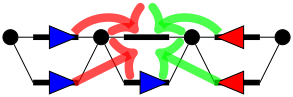
With solving for optimality ruled out, common approaches for railway scheduling proceed by "rolling out" schedules over time [Khadilkar, 2018; Prasad et al., 2021]. Abstractly, such algorithms begin from an initial state in which trains are located in respective resources. Then, at each time step, a train is chosen from those eligible to move, and moved forward. This process is continued until (possibly) all the trains complete their journeys. Since the decision of which train to move at each step is made myopically, there is a possibility of reaching a deadlock state, from which no further progress is possible unless some train moves backward-which is expensive and induces large delays in practice. Figure 1 shows a network with three resources, with one free track in the middle resource. If a train heading right is moved into this free track, there is a deadlock. However, deadlock can be avoided by moving a train heading left into the free track.
Interestingly, detecting deadlocks in the general JSSP is also NP-complete [Araki et al., 1977; Cocco and Monasson, 2001]. It has consequently been accepted wisdom in the railway scheduling community [T¨ornquist and Persson, 2007; Pachl, 2012; Khadilkar, 2017b; Vujanic and Hill, 2022] that deadlock detection for railway scheduling is also NPcomplete in all its forms. The motivation for our work is a result by Reveliotis et al. [1997] for a variant of JSSP called single-unit resource allocations systems (SURAS), showing that in many reasonable situations and for an arbitrary network topology, a necessary and sufficient condition for deadlock detection can be computed in polynomial time.
We make an explicit connection between the SURAS polynomial-time deadlock detection condition given by Reveliotis et al. [1997] and the railway scheduling problem. In the case where every resource (station and track section) has at least two tracks, we show that this condition can be evaluated for arbitrary network states with a linear complexity in the number of trains (slightly more efficiently than Reveliotis et al.). Thereafter, we demonstrate the significant benefit of implementing not just sufficient but necessary conditions for deadlock-free movement on real-world railway networks in India. These include single-track as well as multi-track lines, thus showcasing the wide applicability of the algorithm.
From an infrastructure perspective, laying two tracks has only modest additional cost compared to laying one track, because the land and utilities infrastructure already exists. Hence the only places where single tracks are typically laid are ones where the traffic is low (in which case sophisticated algorithms are not needed) or where the terrain is tough. Indeed it is apparent even from data sets used in the academic literature [Pappaterra et al., 2021; Prasad et al., 2021] that nodes in real-world railway lines usually contain more than one track. Even where single tracks exist (we have empirical results in Section 5), we can handle them so long as a set of feasible moves exist for moving trains to the nearest multi-track resource. At this point, we can drop empty single tracks from the analysis (since they effectively connect two resources, rather than act as independent resources) and the remaining analysis is valid. In the case of scheduling algorithms, we simply ensure that a train that moves into a single track must be moved on to a multi-track section before another train move is attempted.
After discussing related work in Section 2, we formalise the railway deadlock detection problem in Section 3. In Section 4, we present a novel and conceptually simple interpretation of the detection rule of Reveliotis et al. [1997] for multitrack networks. In Section 5, we empirically validate the utility of this rule in scheduling. We conclude in Section 6.
2 RelatedWork
The railway scheduling problem is that of establishing a feasible timetable for a set of 'services' between given origins and destinations [T¨ornquist and Persson, 2007]. Previous work [Cai and Goh, 1994; Liu and Kozan, 2009; Strotmann, 2007] shows that the Job Shop Scheduling Problem (JSSP) and railway scheduling are reducible to each other; their decision variants are both NP-complete. The train scheduling problem can be solved at leisure, combining exact and randomised search algorithms [Higgins et al., 1996; T¨ornquist and Persson, 2007]. The train rescheduling problem involves a disruption externally imposed on the timetable, from which one must quickly compute a set of recovery actions to return to the original timetable [Sinha et al., 2016]. Delays in this context can be computed relative to the corresponding event times in the original timetable. Deadlocks are also important in this context since disruptions to the timetable may require changes in the order of train moves, with uncertain implications for operational feasibility. In this paper, we consider both scheduling and rescheduling, with the understanding that computational complexity has more impact on rescheduling (disruption recovery) than on scheduling (timetabling).
Rescheduling and Deadlock Avoidance in Railways. While exact formulations of rescheduling as an optimisation problem are available [Higgins et al., 1996; T¨ornquist and Persson, 2007], they are not scalable. Practical approaches instead use heuristics [Higgins et al., 1997; Chen et al., 2015] or pretrained policies [ ˇSemrov et al., 2016; Khadilkar, 2018; Prasad et al., 2021] to move trains forward through the network (in a manner analogous to checkers pieces) until they reach their destinations. The order of train movements, their timings, and track allocations vary by the algorithm. However, as illustrated in Figure 1, the risk in all such finitelookahead methods is that of deadlock, or a situation where some or all trains are unable to move forward because of a circular dependence on each other [Pachl, 2012].
Pachl [2012] proposes four conditions which are necessary to create deadlocks. If a scheduling strategy ensures that at least one of these conditions is not met, it is sufficient to avoid deadlocks. Similarly, Mackenzie [2010] proposes sufficient conditions for avoiding deadlock, including the conservative path-to-destination approach. Khadilkar [2017b] proposes the critical-first approach for railway lines, which focuses on prioritising occupants of the most constrained resources in order to avoid bottlenecks. The condition in this case is to keep moving trains forward until at least one additional free track is available for other trains to pass. Vujanic and Hill [2022] make this more concrete by defining the notion of a safe state as one where all nodes (resources) have an unoccupied slot. If initialised from a compliant initial state, their procedure takes polynomial time for scheduling.
The basis for all these studies is that the NP-completeness of the general deadlock detection problem makes it hard to detect deadlocks in instances encountered in practice. Therefore, deadlock detection is typically performed by rules that provably detect deadlocks, but might also flag false positives. The novelty of our paper is in identifying the applicability of an optimal polynomial-time deadlock detection algorithm in JSSP to the railway context (the notion of optimality is formally defined below).
Deadlock Avoidance in JSSP. We shall first define the various terms used in this paper. The problem of evaluating an arbitrary state of the railway network, for the presence/absence of present/future deadlock, is deadlock detection. Any subsequent scheduling policies that reduce the probability of deadlock (but not eliminate it) are called deadlock avoiding policies, while scheduling policies that guarantee the absence of deadlock are called deadlock free policies.
Similar to the railway scheduling case, it is well known that optimal deadlock detection in JSSP is also NP-complete. Araki et al. [1977] consider the question: "given a state S, is S safe?" They reduce the 3-SAT problem [Cocco and Monasson, 2001] to optimal deadlock detection in JSSP, thereby proving the latter to be NP-complete. Fanti et al. [1997] derive necessary and sufficient conditions for deadlock in production systems with resource sharing, and then propose a 'restriction policy' that is tractable and provably correct (in the sense of sufficiency). Gold [1978] considered the question from a more practical perspective, examining under what restrictions on state S one can efficiently detect deadlock. They derived some conditions under which deadlock detection can be solved in polynomial time.
Optimal Deadlock Detection. Previously published studies also consider two forms of optimality in the present context. The first definition of optimality implies the minimisation of delays in the schedule with respect to a reference timetable, or the minimisation of the makespan of the schedule if no reference timetable is available [T¨ornquist and Persson, 2007]. The second definition of optimality [Reveliotis et al., 1997] refers to the removal of unsafe transitions from the current state, with the objective of identifying the smallest (hence optimal) set of unsafe transitions that ensures the absence of present or future deadlocks. In this paper, by optimal rule we refer to the second definition: to a rule that characterises necessary and sufficient conditions of states or transitions to be safe, and hence can be used for deadlock-free scheduling.
Reveliotis et al. [1997] develop necessary and sufficient conditions for deadlock prevention in "single-unit sequential resource allocation systems" (SURAS). They show that deadlock detection in polynomial-time is possible in the special case where every resource in the system has a minimum capacity of 2 units. If the number of resources is m and ¯ C is the maximum capacity among these nodes, their detection condition has O(m2 ¯ C) complexity. The intuition behind this number is that a search algorithm makes m passes through the set of m resources, eliminating one eligible resource in each pass. Our observation is that this result applies to the case of arbitrary railway network topologies (branching and straight lines) as long as there are at least two tracks in each node (in railway terminology, at stations and inter-station track sections). Furthermore, (i) the result can actually be implemented in linear (and not quadratic) complexity, and (ii) we can handle single-resource nodes under reasonable assumptions, as explained in Section 1.
3 Deadlock Detection
In this section, we specify the problem of (optimal) deadlock detection. We begin from the broader context of railway scheduling, within which this problem arises.
3.1 Railway Scheduling Problem
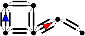
Railway Infrastructure. A railway network is made up of a number of resources, each containing some number of parallel tracks running from one end of the resource to the other. Tracks admit traffic in both directions. Stations (where trains may halt) as well as the inter-station track sections between them (where trains do not have scheduled halts) are modeled as resources. A resource connects to other resources through one of its ends. Typically, terminal resources have all their connections only from one end, but in general we could have cycles in the network topology. Figure 2 shows an illustrative railway network with branching and a cycle; the example in Figure 1 has a linear topology (often called a line).
Desired Schedule. The dynamic aspect of the scheduling problem arises from the movement of a set of trains through resources. The target is to meet a desired schedule Sdesired, which may be represented as a set of N events:
Event e[i] specifies that train train[i] must be moved from resource start res[i] to the adjoining resource next res[i] at time time[i]. Now, it may not be possible to execute Sdesired, due to constraints imposed by the railway infrastructure. For instance, if three events all mean to push trains into the same resource at the same time, but this resource only has two free tracks, then at least one of the events will have to be delayed. The goal of scheduling is to compute an operable schedule Soperable that is feasible to execute, but at the expense of delaying a subset of events in Sdesired. For each event e[i], the operable schedule has a replacement e[i] with a new time time[i] ≥ time[i]:
Formally, the objective function to be minimised while computing Soperable is the average departure delay
Since the problem of computing an operable schedule that minimises ADD is NP-hard [Mascis and Pacciarelli, 2002], one practical alternative is to roll out schedules over time, ensuring operability, while making greedy choices to reduce delays [Khadilkar, 2018; Prasad et al., 2021].
3.2 Roll-Out Algorithms
A roll-out algorithm executes the set of events {e[i], 1 ≤ i ≤ N} one by one. The algorithm begins with a counter τ set to the earliest event time, with state sτ associating each train with its initial resource. An event i is said to be executed (and inserted into Soperable) when the algorithm sets time[i].
At each counter value τ, the algorithm compiles the list of events that are eligible: these are events e[i], 1 ≤ i ≤ N, such that (i) train[i] is in start res[i] in state sτ ; (ii) there is a free track in resource next res[i] in sτ ; and (iii) time[i] ≥ τ. If, indeed, there are eligible events, one of these events i is selected and executed by setting time[i] = τ. The updated event e[i] is moved into Soperable, and e[i] is no longer eligible. As long as there are eligible events at τ, these are repeatedly executed, until there are no eligible events at τ; in this case τ is incremented and the procedure continues. Since train journeys are a sequence of contiguous resources, any train can be in at most one eligible event at any time step. Hence, it is sometimes convenient to view the set of eligible events at τ as the set of trains that are eligible to be moved at τ.
By construction, the set of events that have already been executed by a roll-out algorithm have no internal conflicts. Hence, if all N events in Sdesired get executed, we are guaranteed an operable schedule Soperable. However, the ADD of Soperable depends on the delays introduced while executing the events. The choice of which event among the eligible ones to execute at any step also has the long-term consequence of which events become eligible in subsequent time steps. By and large, roll-out algorithms make this choice greedily [Khadilkar, 2018; Prasad et al., 2021]. An unfortunate consequence is the possibility of a deadlock, wherein there remain events to execute, but these cannot become eligible at the current counter value τ or anything larger.
3.3 Deadlock Detection Problem
Abstractly, the progress of a roll-out algorithm for generating a schedule can be viewed as a sequence of state transitions. The background data from the problem instance, which guide and constrain these transitions, are (1) the set of resources U; (2) resource capacities encoded by ¯ C : U → N; (3) the set of trains T; and (4) the set of train journeys D = {(t, u1 , u2 , . . . , ult ), t ∈ T}. In D, each journey (t, u1 , u2 , . . . , ult ) contains a train t ∈ T and the identities of some lt ≥ 1 resources through which t must pass in sequence. Exact event times are not needed for deadlock detection. As motivated in Section 1, we make the following "multi-track" assumption while devising and analysing our algorithm, which is presented in Section 4.
However, the problem statement presented below does not depend on this assumption.
States, Actions, Transitions. Each state s in our system contains a subset of trains T ′s ⊆ T that are yet to complete their journeys. In s, each train t ∈ T ′s is in some resource u ∈ U. Hence, a state can be represented as a set of pairs (t, u) ∈ T × U. Let S denote the set of all states. The desired terminal state s⊤ ∈ S is the one in which all trains have reached their destinations. Destinations typically connect to "yards" with effectively infinite capacity, so trains do not occupy regular tracks at their destinations. Hence s⊤ = ∅.
A useful quantity to associate with each state s ∈ S is its "potential" φ(s), which we define to be the sum of the distances of the trains present in s to their respective termini.
Concretely, suppose s = {(ti, ui), 1 ≤ i ≤ m}, where the remaining sequence of resources for train ti to visit after departing ui is u1i , u2i , . . . , uℓi i for some ℓi ≥ 1. Then we have φ(s) = ∑mi=1 (1 + ℓi) . Observe that φ(s⊤) = 0.
The set of actions available from state s ∈ S is denoted A(s). Each action a ∈ A(s) corresponds to moving some train from its current resource to the next one on its journey. Naturally, only moves corresponding to eligible events are present as actions in A(s).
When an action from A(s) is performed on state s ∈ S, we denote the resulting state s + a. Suppose action a ∈ A(s) moves train t in s, where t is in resource u, to its next resource u′ . If u′ is the terminal resource for t, then s+a = s\{(t, u)}; otherwise s + a = (s \ {(t, u)}) ∪ {(t, u′ )}. Notice that when an action from A(s) is performed on s, progress is achieved in the sense that φ(s + a) = φ(s) - 1. Since trains cannot move backwards, this progress cannot be undone. However, as we see next, an action may lead to a state from which further progress is not possible.
Safe and Unsafe States. By definition, the desirable terminal state s⊤ = ∅ is a safe state; so also is every state for which there exists a sequence of actions to reach s⊤. We may write down recursively: for s ∈ S,
This recursive definition gives rise to a straightforward procedure to compute SAFE(s), since any state s+a in the RHS has a potential value φ(·) one unit lower than s. However, there is branching by a factor of |A(s)|, implying exponential complexity for a naive implementation. Our main observation, described in the next section, is that SAFE(s) can be computed in time that is only linear in the size of s.
An unsafe state is a state that is not safe. A deadlocked state is a state containing trains, but on which no valid action can be performed. For s ∈ S,
Since our system contains a finite number of trains, and their journeys are also finite, it follows that φ(·) has a finite upper bound. Since φ(·) decreases by 1 unit after each action, the length of any action sequence starting from any initial state s0 is also guaranteed to be finite. It follows that if s is unsafe, then any sequence of actions starting from s will lead to a deadlocked state, from which no further actions are available.
Computational Problem. We require a procedure that can efficiently identify whether a given state s ∈ S is safe or not. It is convenient to view this procedure as a rule or proposition R(s), which evaluates to a boolean value. R(s) may depend both on s and on the journey details of the trains in D, but must be efficient to compute. Several "sufficient" rules R from the literature guarantee that R(s) =⇒ SAFE(s). We require a "necessary and sufficient" rule, also called an optimal rule, which satisfies R(s) ⇐⇒ SAFE(s).
As described in Section 1, optimal rules are computationally hard on unrestricted problem instances. On the other hand, we show next that if Assumption 1 is satisfied, then an optimal rule can be implemented in only linear time.
4 Linear-Time Algorithm
The algorithm presented here is due to Reveliotis et al. [1997], who proposed it in the context of resource allocation and implemented it with quadratic complexity. We describe this algorithm from the perspective of deadlock detection in railway networks, using the vocabulary introduced in Section 3. We provide a concise proof of correctness based on a graph-theoretic model, and also show that a linear-time implementation is possible.
Next-Stop Graph. The main data structure involved in specifying R0 is a directed graph constructed based on input state s. The construction also requires the resource capacities encoded by ¯ C and the set of train journeys D. We denote this directed graph Gs = (V, E, C), where V is the set of vertices, E the set of edges, and C : V → {red, black} a function that associates a colour with each vertex.
Recall that Ts is the set of trains in s. A resource u ∈ U is a vertex v ∈ V in Gs if and only if u is the current resource for some train t in s, or it is the next resource for some train t in s (as specified in t's journey in D). The colour C(v) of a vertex v ∈ V is red if the corresponding resource has at least one free track (that is, the number of trains in this resource is strictly smaller than the capacity). Fully-occupied vertices are coloured black. Each train t in state s gives rise to an edge from the vertex of its current resource u to the vertex of its next resource u′ . Hence, each edge e ∈ E corresponds to one or more trains in s. Notice that every vertex v ∈ V must have at least one edge, either incoming or outgoing (but possibly one or more of each type).
Surprisingly, one does not need to access the extended journeys of trains in s in order to construct Gs: one only needs the trains' current and next resources. For this reason, we may refer to Gs as the "next-stop graph" of s. Notice that the number of edges in Gs is at most the number of trains in s: that is, |E| ≤ |T|. Clearly Gs does not exceed the size of s or of the journey data D beyond a constant factor, as both s and D use Ω(|T |) space. Even so, Gs provides all the information required for optimal deadlock detection.
Optimal Rule. Our rule R0 has an intuitive form.
Definition 2. For s ∈ S, R0(s) is the proposition: "In Gs, every black vertex has a directed path to some red vertex."
We formally show that under the multi-track assumption, R0 is an optimal deadlock detection rule.
Theorem 3. If the problem instance satisfies Assumption 1, then for s ∈ S, R0(s) ⇐⇒ SAFE(s).
Proof. Let Gs = (V, E, C). We prove the theorem by induction on φ(s). As base case, consider arbitrary s ∈ S for which φ(s) = 1. If so, there is exactly one train t in the network, in a resource that connects to t's terminus. Clearly s is safe since t can be moved into its terminus (thus s transitions into s⊤). Also notice that in this case, Gs comprises exactly two vertices r1, r2 ∈ V , with an outgoing edge from r1 to r2. Since each resource has at least two tracks, r1 and r2 must both be red, making R0(s) trivially true. In short, when φ(s) = 1, R0(s) and SAFE(s) are both true, and thereby equivalent.
Our induction hypothesis is that for some integer m ≥ 1, R0(s) ⇐⇒ SAFE(s) for all s ∈ S having φ(s) = m. Now consider a state s ∈ S for which φ(s) = m+ 1. We separately prove the two implications in the theorem.
- Proof of R0(s) =⇒ SAFE(s). Suppose that R0(s) is true: that is, in Gs, every black vertex has a directed path to some red vertex. We consider two complementary subcases.
1.1. Suppose Gs contains some red vertex r ∈ V with no outgoing edges (Figure 3a). As in our base case, r must contain an incoming edge from some vertex v ∈ V . Notice that r has two or more empty tracks. Hence, we can move a train t from v to r to obtain a state s′ with φ(s′ ) = m. If there are any incoming edges into v in s, or v has trains other than t in s, then v would also be a vertex in s′ , but now coloured red. Otherwise v would not be a vertex in Gs′ . Depending on t's next stop from s′ , r could get a new edge to an existing vertex or a new red vertex in Gs′ . Regardless, notice that if any black vertex had a path to a red vertex in Gs, it would continue to have a path to a red vertex in Gs′ . Hence, if R0(s) is true, then R0(s′ ) is also true. By the induction hypothesis, s′ is safe, and hence s is also safe.
1.2. The second subcase is that every red vertex in Gs has an outgoing edge (Figure 3b); every black vertex in Gs will anyway have at least one outgoing edge. In this case, we consider a subgraph G′ of Gs (Figure 3c), which differs only in the set of edges. Indeed let G′ = (V,E′ ,C) so that (i) each vertex v ∈ V has exactly one outgoing edge in E′ , and (ii) each black vertex in G′ has a directed path to some red vertex in G′ . A natural way to construct E′ would be to first fix some outgoing edge to a red vertex from all black vertices having such an edge in E, then to fix an outgoing edge to one of those black vertices from all other black vertices having such an edge in E, and proceeding similarly until all black vertices have an outgoing edge. Thereafter each red vertex can be given an arbitrary outgoing edge from E.
By its definition, G′ cannot have a directed cycle with only black vertices (since that would imply that those vertices do
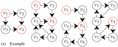
- (b) Example of Gs in which all red vertices have an outgoing edge.
(a) Example of Gs containing a red vertex with no outgoing edges.
(c) G′ constructed for Gs from Figure 3b.
(d) Example of Gs with black vertices not having a path to any red vertex.
Figure 3: Graphs illustrating cases in proof of Theorem 3.
not have a directed path to some red vertex in G, hence invalidating R0(s)). Also, since it has an outgoing edge for each vertex, G′ must contain a directed cycle. In summary, we infer that G′ must contain a directed cycle with at least one red vertex. Indeed let such a cycle C contain the sequence of vertices r, v1, v2, . . . , vm for some m ≥ 1, where r is a red vertex. We are indifferent to the colours of v1, v2, . . . , vm.
Now consider the action of moving a train t from vm to r, leading to next state s′ . The set of vertices in Gs′ remains identical to that of s, except that Gs′ may get a new red vertex that is the next stop for t in s′ . The set of edges in Gs′ is also identical to that of Gs, except for (i) the possible loss of the single edge from vm to r in case t was the only train having that transition in s, and (ii) the possible gain of a new outgoing edge from r. Regardless, vm is necessarily a red vertex in Gs′ , and moreover, any black vertex that had a directed path to r in Gs must have a path to vm in Gs′ (since r has a path through the sequence of vertices in C to vm). Directed paths not involving C in Gs remain the same in Gs′ . Hence, we conclude that if R0(s) is true, then R0(s′ ) is also true. Since φ(s′ ) = m, we obtain from the induction hypothesis that s′ is safe. Since we can go from s to s′ by moving t, we observe that s must also be safe.
2. Proof of SAFE(s) =⇒ R0(s). Suppose R0(s) is not true: that is, there exists a black vertex b ∈ V with no directed path to any red vertex in V (Figure 3d). b is fully occupied in s, and so it must have outgoing edges in Gs. Since these edges to do not lead to a red vertex in Gs, we surmise that there exists a finite subset of black vertices B ⊆ V of size at least two such that for each vertex in B, all outgoing edges lead to other vertices in B. Since every vertex b′ ∈ B is fullyoccupied, no train can be moved out from or moved into any vertex in B. If s is already in deadlock, by definition it is unsafe. On the other hand, after any possible move of any train outside of B in s to reach s′ , B remains a finite set of black vertices in Gs′ , with no directed path to any red vertex. Since φ(s′ ) = m, the induction hypothesis gives us that s′ is unsafe, and hence s is unsafe.
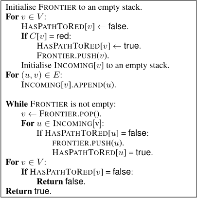
Although R0 is essentially a rephrasing of the rule given by Reveliotis et al. [1997] for SURAS, its interpretation in terms of a next-stop graph Gs is novel. The algorithm given by Reveliotis et al. [ 1997] eliminates one node in each pass through the set of resources, hence takes time that is quadratic in the number of resources. On the other hand, it is easy to see that R0(s) can be computed in time that is only linear in the number of edges in Gs, which is generally much smaller than |U|2 . The pseudocode in Figure 4 is for an implementation of R0 by a standard search algorithm [Russell and Norvig, 2022, see Chapter 3], taking O(|E|) operations for input Gs = (V, E, C).
5 Experimental Validation
We compare our proposed rule R0 against other deadlock avoidance algorithms on real railway schedules as well as synthetically-generated ones. Data and code to reproduce the results reported in this section are available at https: //github.com/Hastyn/Linear-Time-Deadlock-Detection/.
5.1 Data Description
We use published timetables and infrastructure information from three portions of the Indian Railway network. These portions are fromAjmer (northwest India), Kanpur (north India) and Konkan (west coast). Of these, Ajmer and Kanpur are predominantly multi-track at stations as well as the connecting sections between stations, while Konkan has multitrack stations but mostly single-track connecting sections (we handle this scenario by moving trains from one station to the next without stopping in the connecting sections, as outlined earlier). Details from these networks are summarised in Table 1. In addition to the real data sets, we also generate 8 hypothetical lines and branching networks to have better control on the characteristics. HYP-1 is a small toy dataset, HYP-2 and HYP-3 share the same infrastructure, but HYP-3 has twice the number of trains of HYP-2. HYP-4 and HYP-5 simulate very high traffic networks with only four stations but a large number of trains. HYP-6, HYP-7, and HYP-8 are branching networks with HYP-7 having high traffic. In Table 1, the density reported is the total number of events occurring per minute per resource in the network.
| Instance | Sn. | Tns. | Time Span | Events | Con. Sec. | Density |
|---|---|---|---|---|---|---|
| Ajmer | 52 | 444 | 5.5 day | 13129 | 51 | 0.016 |
| Kanpur | 27 | 190 | 1.4 day | 3858 | 26 | 0.036 |
| Konkan | 59 | 85 | 2.2 day | 2709 | 58 | 0.007 |
| HYP-1 | 5 | 8 | 1.8 hrs | 40 | 4 | 0.041 |
| HYP-2 | 11 | 60 | 2.0 day | 660 | 10 | 0.011 |
| HYP-3 | 11 | 120 | 2.1 day | 1320 | 10 | 0.021 |
| HYP-4 | 4 | 350 | 0.8 hrs | 1290 | 3 | 3.839 |
| HYP-5 | 3 | 200 | 0.5 hrs | 4766 | 2 | 31.773 |
| HYP-6 | 6 | 6 | 0.8 hrs | 23 | 5 | 0.044 |
| HYP-7 | 26 | 500 | 3.0 hrs | 4537 | 27 | 0.476 |
| HYP-8 | 22 | 100 | 4.8 hrs | 1046 | 21 | 0.084 |
5.2 ComparisonWith Baselines
The goal of our experiments is to test the reduction in ADD (defined in (1)) as a result of dividing the action set in any given state optimally into safe and unsafe labels. Considering this to be a binary classification problem, we pick one baseline rule Rg which allows false negatives (marking an actually unsafe state as safe) and one rule Rc which allows false positives (marking an actually safe state as unsafe). We note that the rules Rg and Rc correspond to 'greedy' [Prasad et al., 2021] and 'critical first' [Khadilkar, 2017b] in their original forms. Briefly, the greedy algorithmmarks a train movement as safe if it has at least two feasible forward moves. Critical-first is a sufficient condition for deadlock free movement, which allows a train to move ahead as long as it only stops in a resource where at least one additional track is free. For every compounded set of primitive moves, this results in a state where every resource has at least one free track.
The critical first algorithm further provides a ranking order when multiple train movements are marked as safe, based on the number of presently free tracks in the resource the train is currently occupying (criticality of the node). We use this logic to rank train moves among the set marked safe by each rule. The resulting ADD for all problem instances and algorithms is summarised in Table 2. We emphasise that only the safe action masking (by using R0, Rg, or Rc) differs among the algorithms, and the remaining scheduling/rescheduling policy is the same. In order to generate statistical results, we generate perturbed versions of each instance by moving the entire journey of each train in the reference timetable by an amount picked uniformly at random in [-30, 30] minutes. Refer to Prasad et al. [2021] for details of the perturbations.
From Table 2, we first confirm that both Rc (sufficient) and R0 (necessary and sufficient) conditions result in deadlockfree schedules for all instances. Second, R0 performs significantly better than Rc in all instances, in terms of schedule efficiency. This demonstrates the advantage of employing an optimal deadlock detection condition. Rg outperforms R0 in three instances, all of which have low traffic density (see Table 1). However, the ADD for R0 is competitive even in these instances. On the other hand, Rg deadlocks in instances with high traffic density, and hence in general would not be a suitable choice for real-time rescheduling.
| Instance | Critical First (Rc) | Greedy (Rg) | R0 |
|---|---|---|---|
| Ajmer | 4.76±0.07 | 4.19±0.08 | 4.12±0.09 |
| Kanpur | 1.35±0.07 | 3.57±0.09 | 1.29±0.05 |
| Konkan | 60.33±0.69 | 42.22±0.59 | 42.60±0.51 |
| HYP-1 | 19.30±1.74 | 16.22±1.29 | 16.49±1.30 |
| HYP-2 | 6.33±0.33 | 4.29±0.21 | 4.31±0.21 |
| HYP-3 | 7.02±0.91 | 5.01±0.16 | 0.83±0.07 |
| HYP-4 | 1773.73±12.79 | deadlock | 1170.11±2.46 |
| HYP-5 | 654.9±17.26 | 568.07±2.71 | 524.23±2.39 |
| HYP-6 | 12.07±1.43 | deadlock | 6.42±1.20 |
| HYP-7 | 1487.88±22.11 | deadlock | 1228.30±1.61 |
| HYP-8 | 776.96±27.74 | 215.74±2.04 | 169.48±1.90 |
5.3 Policy Improvement
As a second experiment, we consider the effect of optimal deadlock detection on the efficiency of resulting schedules, by performing policy improvement using roll-outs [Tesauro and Galperin, 1996; Agarwal, 2022]. Under policy improvement, a base schedule is progressively improved by updating each action to one that minimises delay when followed by a roll-out policy. In Table 3, we start with the schedule produced by R0 in Table 2 for all three algorithms (for a fair comparison). For every decision taken in the sequence, we roll out the individual trajectories for all alternative actions which are also marked as safe by the relevant rule. We choose the schedule with the least ADD out of these results, move to the next decision in the sequence, and repeat. The results in Table 3 show that the rollouts using R0 (which provides the maximal set of feasible actions) are predominantly more effective than those using Rc and Rg. In some cases, Rc and Rg are unable to improve on the baseline schedule given by R0, while R0 results in improvement over Table 2 in all instances.
6 Conclusion
In this paper, we show that in contrast to the accepted characterisation of railway scheduling in the literature, a polynomial-time deadlock detection method from the resource allocation literature applies to a large class of (re)scheduling problems. Our version of the implementation is in fact linear-time for arbitrary network topology, so long as each resource (station or connecting section) has at least two tracks. Further, we show that under a mild assumption (availability of a sequence of moves to bring all trains in singletrack resources to a multi-track resource), we can also handle scheduling in the single-track scenario. Our empirical results show that using an optimal deadlock detection strategy significantly improves scheduling efficiency, in addition to providing feasibility guarantees. One important open question for the future is to evaluate the usefulness of optimal action masking while training data-driven scheduling policies.
| Instance | Rg Rollout | Rc Rollout | R0 Rollout |
| Ajmer | 3.43±0.04 | 3.79±0.05 | 3.43±0.07 |
| Kanpur | 1.29±0.05 | 1.13±0.05 | 1.09±0.05 |
| Konkan | 39.67±0.57 | 42.59±0.51 | 40.24±0.61 |
| HYP-1 | 15.75±1.26 | 16.18±1.28 | 15.74±1.26 |
| HYP-2 | 3.99±0.24 | 4.19±0.18 | 4.08±0.20 |
| HYP-3 | 0.83±0.07 | 0.82±0.07 | 0.74±0.06 |
| HYP-4 | 1170.11±2.46 | 1170.11±2.46 | 1166.26±2.49 |
| HYP-5 | 524.23± 2.39 | 524.23± 2.39 | 517.23±2.09 |
| HYP-6 | 6.35±1.22 | 5.90±1.01 | 4.20±0.62 |
| HYP-7 | 1215.73± 1.57 | 1228.3±1.61 | 1225.99±1.36 |
| HYP-8 | 169.48±1.90 | 169.48±1.90 | 165.79±2.42 |
Acknowledgements
We thank Spyros Reveliotis for sharing full versions of relevant literature that was otherwise not available. We thank Abhiram Ranade from IIT Bombay for informative discussions, and Shripad Salsingikar from TCS for providing railway data.
@inproceedings{ijcai2024p641,
  title     = {Linear-Time Optimal Deadlock Detection for Efficient Scheduling in Multi-Track Railway Networks},
  author    = {Doshi, Hastyn and Tripathi, Ayush and Agarwal, Keshav and Khadilkar, Harshad and Kalyanakrishnan, Shivaram},
  booktitle = {Proceedings of the Thirty-Third International Joint Conference on
               Artificial Intelligence, {IJCAI-24}},
  publisher = {International Joint Conferences on Artificial Intelligence Organization},
  editor    = {Kate Larson},
  pages     = {5799--5807},
  year      = {2024},
  month     = {8},
  note      = {Main Track},
  doi       = {10.24963/ijcai.2024/641},
  url       = {https://doi.org/10.24963/ijcai.2024/641},
}
TY - CPAPER TI - Linear-Time Optimal Deadlock Detection for Efficient Scheduling in Multi-Track Railway Networks AU - Doshi, Hastyn AU - Tripathi, Ayush AU - Agarwal, Keshav AU - Khadilkar, Harshad AU - Kalyanakrishnan, Shivaram T2 - Proceedings of the Thirty-Third International Joint Conference on Artificial Intelligence, IJCAI-24 PB - International Joint Conferences on Artificial Intelligence Organization PY - 2024 SP - 5799 EP - 5807 DO - 10.24963/ijcai.2024/641 UR - https://doi.org/10.24963/ijcai.2024/641 ER -Copied
Machine-readable versions of this paper, for tools and AI agents:





