
Proportion-based Sensitivity Analysis of Uncontrolled Confounding Bias in Causal Inference
Proceedings of the Thirty-Third International Joint Conference on Artificial Intelligence. Main Track. Pages 7136-7143.
https://doi.org/10.24963/ijcai.2024/789
Keywords
- Uncertainty in AI: UAI: Causality, structural causal models and causal inference
Abstract
Uncontrolled confounding bias causes a spurious relationship between an exposure variable and an outcome variable and precludes reliable evaluation of the causal effect from observed data.Thus, it is important to observe a sufficient set of confounders to reliably evaluate the causal effect.However, there is no statistical method for judging whether an available set of covariates is sufficient to derive a reliable estimator for the causal effect.To address this problem, we focus on the fact that the mean squared error (MSE) of the outcome variable with respect to the average causal risk can be described as the sum of "the conditional variance of the outcome variable given the exposure variable" and "the square of the uncontrolled confounding bias".We then propose a novel sensitivity analysis, namely, the proportion-based sensitivity analysis of uncontrolled confounding bias in causal effects (PSA) in which the sensitivity parameter is formulated as the proportion of "the square of the uncontrolled confounding bias" to the MSE, and we clarify some properties.We also demonstrate the applicability of the PSA through two case studies.
- [Balke and Pearl, 1997] Alexander Balke and Judea Pearl. Bounds on treatment effects from studies with imperfect compliance. Journal of the American Statistical Associa- tion, 92(439):1171-1176, 1997.
- [Balke, 1995] Alexander Balke. Probabilistic Counterfac- tuals: Semantics, Computation, and Applications. Ph.D. Thesis, University of California, Los Angeles, 1995.
- [Cai et al., 2007] Zhihong Cai, Manabu Kuroki, and Tosiya Sato. Non-parametric bounds on treatment effects with non-compliance by covariate adjustment. Statistics in Medicine, 26(16):3188-3204, 2007.
- [Cai et al., 2008] Zhihong Cai, Manabu Kuroki, Judea Pearl, and Jin Tian. Bounds on direct effects in the pres- ence of confounded intermediate variables. Biometrics, 64(3):695-701, 2008.
- [Cinelli and Hazlett, 2020] Carlos Cinelli and Chad Hazlett. Making sense of sensitivity: Extending omitted variable bias. Journal of the Royal Statistical Society Series B- Statistical Methodology, 82(1):39-67, 2020.
- [Greenland, 2003] Sander Greenland. The impact of prior distributions for uncontrolled confounding and response bias: a case study of the relation of wire codes and mag- netic fields to childhood leukemia. Journal of the Ameri- can Statistical Association, 98(461):47-54, 2003.
- [Greenland, 2005] Sander Greenland. Multiple-bias mod- eling for analysis of observational data. Journal of the Royal Statistical Society: Series A (Statistics in Society), 168(2):267-306, 2005.
- [Imbens and Rubin, 2015] Guido W. Imbens and Donald B. Rubin. Causal Inference in Statistics, Social, and Biomed- ical Sciences. Cambridge University Press, 2015.
- [Kuroki and Cai, 2008] Manabu Kuroki and Zhihong Cai. Formulating tightest bounds on causal effects in studies with unmeasured confounders. Statistics in Medicine, 27(30):6597-6611, 2008.
- [Kuroki and Miyakawa, 2003] Manabu Kuroki and Masami Miyakawa. Covariate selection for estimating the causal effect of control plans by using causal diagrams. Jour- nal of the Royal Statistical Society: Series B (Statistical Methodology), 65(1):209-222, 2003.
- [Kuroki, 2008] Manabu Kuroki. The evaluation of causal ef- fects on the variance and its application to process anal- ysis. Journal of the Journal of The Japanese Society for Quality Control, 38:407-418, 2008.
- [Kuroki, 2012] Manabu Kuroki. Optimizing a control plan using a structural equation model with an application to statistical process analysis. Journal of Applied Statistics, 39(3):673-694, 2012.
- [Li et al., 2023] Ang Li, Scott Mueller, and Judea Pearl. ϵ- identifiability of causal quantities. Technical Report R- 525, <http://ftp.cs.ucla.edu/pub/stat ser/r525.pdf>, De- partment of Computer Science, University of California, Los Angeles, CA, 2023. Link
- [MacLehose et al., 2005] Richard F MacLehose, Sol Kauf- man, Jay S Kaufman, and Charles Poole. Bounding causal effects under uncontrolled confounding using counterfac- tuals. Epidemiology, pages 548-555, 2005.
- [Manski, 1990] Charles F Manski. Nonparametric bounds on treatment effects. The American Economic Review, 80(2):319-323, 1990.
- [McCandless et al., 2007] Lawrence C McCandless, Paul Gustafson, and Adrian Levy. Bayesian sensitivity anal- ysis for unmeasured confounding in observational studies. Statistics in Medicine, 26(11):2331-2347, 2007.
- [McCandless et al., 2008] Lawrence C McCandless, Paul Gustafson, and Adrian R Levy. A sensitivity analysis us- ing information about measured confounders yielded im- proved uncertainty assessments for unmeasured confound- ing. Journal of Clinical Epidemiology, 61(3):247-255, 2008.
- [Pearl, 2009] Judea Pearl. Causality: Models, Reasoning and Inference. Cambridge University Press, 2nd edition, 2009.
- [Peña, 2022] Jose M Peña. Simple yet sharp sensitivity anal- ysis for unmeasured confounding. Journal of Causal In- ference, 10(1):1-17, 2022.
- [Tian and Pearl, 2000] Jin Tian and Judea Pearl. Probabil- ities of causation: Bounds and identification. Annals of Mathematics and Artificial Intelligence, 28(1-4):287-313, 2000.
- [Tian and Pearl, 2002] Jin Tian and Judea Pearl. A general identification condition for causal effects. In National Conference on Artificial Intelligence, volume 18, pages 567-573. AAAI Press, 2002.
- [VanderWeele and Ding, 2017] Tyler J VanderWeele and Peng Ding. Sensitivity analysis in observational research: introducing the e-value. Annals of Internal Medicine, 167(4):268-274, 2017.
- [VanderWeele et al., 2019] Tyler J. VanderWeele, Peng Ding, and Maya Mathur. Technical considerations in the use of the e-value. Journal of Causal Inference, 7(2):20180007, 2019.
References were extracted automatically from the PDF and may contain errors.
Full text extracted automatically from the PDF; figures, tables and equations may differ. The PDF is the version of record.
1 Introduction
1.1 Background
The evaluation of the causal effect of an exposure variable on an outcome variable is one of the central aims in observational studies. Compared to controlled randomized experiments, observational studies are more susceptible to various types of biases. In particular, uncontrolled confounding bias causes a spurious relationship between the exposure variable and the outcome variable, and this precludes reliable evaluation of the causal effect from observed data. It is well known that such uncontrolled confounding bias arises when there are unmeasured confounders that are associated with both the exposure variable and the outcome variable but are not influenced by them.
When confounders between an exposure variable and an outcome variable are properly measured in observational studies, adjustment methods, such as stratified analysis, can provide a reliable evaluation of the causal effect [Imbens and Rubin, 2015; Pearl, 2009]. However, there is no statistical method to judge whether an available set of covariates is sufficient to derive a reliable estimator of the causal effect because of insufficient knowledge of important confounders or a lack of data on known potential confounders. Sensitivity analyses [Cinelli and Hazlett, 2020; Greenland, 2003; Greenland, 2005; McCandless et al., 2007; McCandless et al., 2008; Pe˜na, 2022; VanderWeele and Ding, 2017; VanderWeele et al., 2019] and bounding methods [Balke, 1995; Balke and Pearl, 1997; Cai et al., 2007; Cai et al., 2008; Kuroki and Cai, 2008; Li et al., 2023; MacLehose et al., 2005; Manski, 1990] have been commonly used to address uncontrolled confounding bias in observational studies.
In this paper, we focus on sensitivity analysis for uncontrolled confounding bias in causal effects. Sensitivity analysis actively introduces covariate information that is not available from observational studies into a statistical causal model as a sensitivity parameter and quantitatively evaluates how the estimate of the causal effect changes when the value of the sensitivity parameter is changed. Therefore, causal judgment using sensitivity analysis is based on the bounds of the causal effect of the exposure variable on the outcome variable (or the uncontrolled confounding bias). Thus, unlike bounding methods, in which the goal is to evaluate the causal effect based on the best-case and worst-case scenarios, sensitivity analysis has the advantage of eliminating unrealistic situations from the causal judgment. However, most of the current sensitivity analyses (i) are formulated based on the mean but not the variation (variance) of the potential outcome variables, and (ii) they do not handle a set of unmeasured confounders that consist of an uncertain number of discrete and continuous variables. Thus, it is reasonable to introduce the uncontrolled confounding bias itself as the sensitivity parameter into sensitivity analysis but not to focus on the association among a specific unmeasured confounder, the exposure variable, and the outcome variable.
1.2 Contribution
In this paper, we focus on the fact that the mean squared error (MSE) of the outcome variable with respect to the average causal risk can be described as the sum of "the conditional variance of the outcome variable given the exposure variable"
and "the square of the uncontrolled confounding bias," i.e., the difference between the conditional mean of the outcome variable given the exposure variable and the average causal risk.
We then propose a novel sensitivity analysis, namely, the proportion-based sensitivity analysis of uncontrolled confounding bias in causal effects (PSA), in which the sensitivity parameter is formulated as the proportion of "the square of the uncontrolled confounding bias" to the MSE of the outcome variable with respect to the average causal risk, and we clarify some properties.
Here, the sensitivity parameters used in the PSA are called the proportion-based sensitivity parameters of uncontrolled confounding bias (PSP).
In contrast to the current sensitivity analysis, the PSA has the following desirable properties.
- (i) The PSA is formulated based on the minimal causal knowledge that (a) the outcome variable cannot have an effect on the exposure variable, and (b) a set of covariates does not occur after the exposure variable or the outcome variable.
- (ii) The PSA enables us to handle a set of covariates that consists of an uncertain number of discrete and continuous variables.
- (iii) The PSP always falls inside the range [0,1] without any assumptions: The PSP can be interpreted as the proportion.
- (iv) The PSP has an estimable cutoff value that qualitatively prevents misleading causal judgment when we use statistical measures, such as statistical risk differences, through observed data to evaluate the causal effect.
In particular, in the framework of linear structural equation models (linear SEMs), the PSP can be interpreted from the viewpoint of the interventional variance that evaluates the variation of the outcome variable when conducting external intervention to the exposure variable [Kuroki, 2008; Kuroki, 2012; Kuroki and Miyakawa, 2003]. In addition, we provide a medical case study from the Cooperative Cardiovascular Project [MacLehose et al., 2005] and an industrial case study on setting up painting conditions of car bodies [Kuroki, 2008; Kuroki, 2012] to discuss the applicability of the PSA. The PSA contributes to addressing the evaluation problems of causal effects in the context of statistical causal inferences. Here, given space constraints, proofs, the details of the case studies and numerical experiments are provided in the Supplementary Material.
2 General Framework
2.1 Preliminaries
This section introduces potential outcome variables used to discuss our problem.
For simplicity, let X and Y be an exposure variable and an outcome variable, respectively. For the values x and y taken by X and Y , respectively, let f(x, y) and f(x) be the joint probability density function of (X, Y )T = (x, y)T and the marginal probability density function of X = x, respectively. Here, the notation "T" stands for a transposed vector/matrix. Then, f(y|x) represents the conditional probability density function of Y = y given X = x, defined as f(y|x) def = f(x, y)/f(x) for f(x) ̸= 0. Especially, in this paper, when we emphasize that X and Y are discrete variables, f(x, y), f(x) and f(y|x) are often replaced by pr(x, y), pr(x) and pr(y|x), respectively. In addition, E(Y )(= µy) and var(Y )(= σyy) are the mean of Y and the variance of Y , respectively. E(Y |x)(= µy.x), var(Y |x)(= σyy.x), cov(X, Y )(= σxy) are the conditional mean of Y given X = x, the conditional variance of Y given X = x, and the covariance between X and Y , respectively. A similar notation is used for the other probability density functions and statistical parameters.
In this paper, we assume that readers are familiar with the basic theory of statistical causal inference [Imbens and Rubin, 2015; Pearl, 2009]. In principle, the i-th of the N subjects has a potential outcome variable Yx(i) that would have resulted if X had been x, denoted as X(i) = x. Yx(i) = y means that "Y takes the value y when X is experimentally set to x for the i-th subject" or the counterfactual statement that "Y would have the value y, had X been x for the i-th subject". For the i-th subject, the potential outcome variable Yx(i) is observed only if X(i) is x. This property is called consistency [Imbens and Rubin, 2015; Pearl, 2009], which is formulated as
We note that the subject ensures a deterministic relationship between X and Y in the semantics of statistical causal inference [Imbens and Rubin, 2015; Pearl, 2009].
In this paper, we assume the stable unit treatment value assumption, which can be summarized as follows: (i) the exposure status of any subject does not affect the outcomes of the other subjects (no interference), and (ii) the exposures of all subjects are comparable (no variation in exposure). Thus, when the N subjects in the study are considered random samples from the population of interest, X(i) and Yx(i) are referred to as the values taken by the random variables X and Yx, respectively. Then, the causal probability density function of Yx = y regarding X = x is represented as f(yx). A similar notation is used for other potential outcome variables and causal probability density functions. Here, E(Yx), which is the mean of Yx, is called an average causal risk of X = x on Y . In this paper, for x ̸= x′ ,
are called a causal risk difference and an uncontrolled confounding bias for X = x, respectively.
When a controlled randomized experiment is conducted and compliance is perfect since X is independent of Yx for any x, f(yx) is identifiable and is given by f(yx) = f(y | x). Here, "identifiable" means that the causal quantities, such as f (yx), can be formulated consistently from the joint probability density function of observed variables. In contrast, when it is difficult to conduct a controlled randomized experiment and only observed data are available, f(yx) is also identifiable according to the conditionally ignorable treatment assignment condition [Imbens and Rubin, 2015], or graphically, the back-door criterion [Pearl, 2009]. In other words, if there exists such a set S of observed covariates that X is conditionally independent of Yx given S for any x, we say that treatment assignment is conditionally ignorable given S, or S is a sufficient set of confounders. Here, a variable that is not affected by X is called a covariate, and confounders are included in a set of covariates. Under the conditionally ignorable treatment assignment condition, f(yx) is identifiable by using S as
Here, E[f (y | x, S)] is the expectation of f (y | x, S) regarding S.
Although there are other identification conditions of causal quantities, e.g., f(yx) that can be used to address our problem [Pearl, 2009; Tian and Pearl, 2002], we do not cover them here because of space constraints.
2.2 The PSP for theWhole Population
For the whole population, let us consider the mean squared error (MSE) of Y with respect to E(YX)
Here, we note that var(Y |X), E(YX) and E(Y |X) are functions of the random variable X. Given MSE(Y, E(YX)), equation (1) shows the bias-variance tradeoff that increasing/decreasing the explanation power of X on Y , var(Y |X), leads to decreasing/increasing the uncontrolled confounding bias, E(Y |X) - E(YX). Here, for simplicity, we proceed with our discussion in situations where covariate information is not available. When covariate information on S is available, equation (1) is replaced by
to proceed with our discussion.
From equation (1), MSE(Y, E(YX)) is represented by the sum of "the conditional variance of Y given X" and "the square of the uncontrolled confounding bias". Then, we propose one of the novel sensitivity parameters, namely, the proportion-based sensitivity parameter of uncontrolled confounding bias for the whole population (w-PSP), as follows:
where we define 0/0 = 0. Notably, the w-PSP does not depend on the values taken by X or Y .
The w-PSP has the following properties.
- (a) The w-PSP always falls inside the range [0, 1] without any assumption. Thus, the w-PSP can be interpreted as the proportion that evaluates how much of the MSE is explained by "the square of the uncontrolled confounding bias".
that is, the w-PSP = 1 implies that MSE(Y, E(YX)) is completely explained by the uncontrolled confounding bias alone, and w-PSP = 0 implies no uncontrolled confounding bias.
In addition, under the condition w-PSP ̸= 1, we note that equation (2) can be transformed into
Then, equation (3) provides the following findings:
- (a) Equation (3) is estimable if the information on the w-PSP is available together with observed data regarding X and Y .
- (b) Noting that E(var(Y |X)) is a positive constant value, equation (3) is a nondecreasing function of w-PSP with a vertical asymptote w-PSP = 1.
The w-PSP plays an important role in sensitivity analysis in linear SEMs. Here, for the given threshold wpsp (< 1), the bounds on E((E(Y |X) -E(YX))2 ) are derived by solving the inequality w-PSP≤ w-psp. The bounds present a range within which causal quantities such as E((E(Y |X) - E(YX))2 ), E(Yx) and E(Yx) - E(Yx′ ) must lie given the validity of the assumptions.
2.3 The PSP for the Subpopulation
In this section, for the subpopulation of subjects who take X = x, we consider the MSE of Y with respect to E(Yx) as follows:
Generally, both var(Y |x) and (E(Y |x) -E(Yx))2 are functions of X = x. Then, the proportion-based sensitivity parameter of uncontrolled confounding bias for the subpopulation X = x (s-PSPx) is formulated as
where we define 0/0 = 0. We note that the w-PSP is constant, but the s-PSPx is a function of x.
Here, the s-PSPx share many mathematical properties with the w-PSP. As with the different properties from the w-PSP, we note that equation (5) can be transformed into
for s-PSPx ̸= 1.
Then, equation (6) includes E(Yx), which cannot be estimated from observed data alone. However, if the information on the s-PSPx is available together with observed data, equation (6) is formulated by
Then, if the sign of E(Y |x)-E(Yx) is known, E(Yx) is identifiable.
For the given threshold s-pspx (< 1), the bounds on E(Yx) are derived by solving the inequality s-PSPx ≤ s-pspx regarding E(Yx). Although equation (7) also provides the bounds on various kinds of causal quantities, such as the causal risk ratio and the causal odds ratio, we focus on the bounds on the average causal risk E(Yx) and the average causal risk difference E(Yx) - E(Yx′ ) for x ̸= x′ .
Letting E(Y 2 |x) be the conditional mean of Y 2 given X = x, the following theorem shows that the s-PSPx has an estimable cutoff value that prevents misleading causal judgment qualitatively even when E(Y |x) is utilized to evaluate E(Yx):
3 Theoretical Examples and Application 3.1 Discrete Model
Theoretical Results
In this section, as a theoretical example, we consider the case where X is a discrete variable. Here, when X is a continuous variable, according to [Balke, 1995] and [Balke and Pearl, 1997], in some situations, it is reasonable to assume that there exists an exposure interval around each X = x, within which a subject's outcome is homogeneous. Under such an assumption, it is possible to apply the discussion in this section. In addition, although Y is assumed to be dichotomous and takes one of {y, y′ } in this section, the multivalued or continuous outcome variable can be easily accommodated in the model by using the event Y ≤ y as a (dichotomous) outcome variable.
Equation (7) provides
✏
In addition, from Theorem 1, if s-PSPx < pr(y|x) holds, then the bounds constructed through equation (11) are informative in the sense that they exclude null (if equation (11) is negative, then the lower bound on pr(yx) should be given by 0 because pr(yx) does not take a negative value). In addition, from Theorem 2, we derive the following theorem:
Theorem 3
✓
✑
The proof is provided in the Supplementary Material. In contrast, referring to equation (7), the following theorem is obtained:
Theorem 2
✓
Under the condition s-PSPx, s-PSPx′ ≤ s-psp (< 1) for
✒
The proof is provided in the Supplementary Material.
✏
Under the condition s-PSPx, s-PSPx′ ≤ s-psp (< 1) for x ̸= x′ , the bounds on pr(yx) - pr(yx′ ) are given by
Especially, if
holds, pr(y|x) - pr(y|x′ ) and pr(yx) - pr(yx′ ) have the same sign.
✒
✏
✑
The proof is provided in the Supplementary Material.
Equation (13) qualitatively implies that the statistical risk difference pr(y|x) - pr(y|x′ ) provides no-misleading causal judgments for pr(yx) - pr(yx′ ).
✑
Here, let nx and nx′ be the number of subjects who take X = x and the number of subjects who take X = x′ , respectively. Under the multinomial distribution, letting ˆl and
| dead within | blacks (z′ ) beta-blocker | whites (z) beta-blocker | ||
|---|---|---|---|---|
| 30 days | no (x′ ) | yes (x) | no (x′ ) | yes (x) |
| no (y′ ) | 4224 | 2143 | 63449 | 34868 |
| yes (y) | 1254 | 60 | 22191 | 1103 |
| total | 5478 | 2203 | 85640 | 35971 |
ˆu be the consistent estimator of the lower and upper bounds of equation (12) using the sample probabilities, ˆ pr(y|x) and ˆ pr(y|x′ ) when a.var(·) represents the asymptotic variance, a.var(ˆl) and a.var(ˆu) are given by
respectively. The derivation is provided in the Supplementary Material.
Here, we note that [Tian and Pearl, 2000] provides the sharp bounds on pr(yx) as
for any x. Then, since the simple bounds on pr(yx) - pr(yx′ ) are given by
Here, equation (17) is called the Tian-Pearl bounds. By combining equation (12) with equation (17), we can derive the bounds that are sharper than those in [Tian and Pearl, 2000] because we have
Case Study: Cooperative Cardiovascular Project
We illustrate our results by using data from the Cooperative Cardiovascular Project [MacLehose et al., 2005]. Table 1 shows the use of beta-blockers and 30-day mortality among acute myocardial infarction patients, stratified by ethnicity (black and white patients). Obviously, it is probable that there exist some other confounders that affect both betablocker users and 30-day mortality, such as sex and disease status. We limit our discussion in this section to the evaluation of the causal risk difference of beta-blocker use on 30day mortality for black patients. For the discussion of white patients, refer to the Supplementary Material.
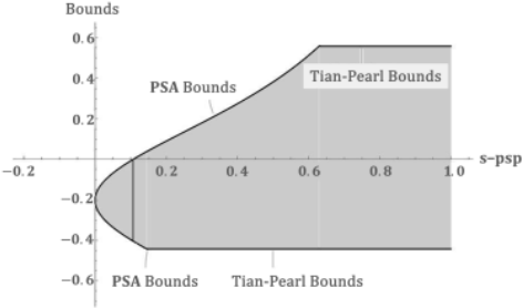
From Figure 1, for s-psp∈ [0.000, 0.107], Theorem 3 shows that the s-psp provides the bounds ([-0.420, 0.000] for s-psp= 0.107) for the black patients who exclude null, which suggests that the beta-blocker must have a preventive effect on 30-day mortality among the black patients. In contrast, the Tian-Pearl bounds provide the range [-0.442, 0.558] regardless of the value of s-psp because the Tian-Pearl bounds do not take the impact of the uncontrolled confounding bias into account. On the other hand, the upper bound based on the s-psp is higher than that of the Tian-Pearl bounds for spsp> 0.629, and the lower bounds based on the s-psp are lower than that of the Tian-Pearl bounds for s-psp> 0.146. Figure 1 shows that beta-blocker use can reduce the 30-day mortality for blacks if s-psp∈ [0.000, 0.107], which does not contradict [Kuroki and Cai, 2008] and [MacLehose et al., 2005]. For details, see the Supplementary Material.
3.2 Linear SEM
Preliminaries
In this section, when it is assumed that cause-effect relationships (data-generating process) between random variables can be represented by a Gaussian linear SEM and the corresponding directed acyclic graph (DAG), we apply the w-PSP to linear SEMs. Here, we refer to nodes in the DAG and random variables of the linear SEM interchangeably throughout this paper. In addition, for the graph-theoretic terminology used in this paper, refer to [Pearl, 2009].
Let us suppose that a DAG G = (V ,E) with a set V = {V1, V2, . . . , Vm} of continuous random variables and a set E of edges is given. G is called a path diagram when each child-parent family in G represents a data-generating process shown in the linear SEM
where pa(Vi) denotes a set of parents of Vi in G (the directed edge Vj → Vi is assigned if Vj is a parent of Vi) and random disturbances εv = (εv1 , εv2 , . . . , εvm )T are assumed to be normally distributed with an m-dimensional zero mean vector and m×m invertible variance-covariance matrix. In addition, the bidirected edges between Vi and Vj (Vi ↔ Vj) are assigned to a nonzero correlation relationship between ϵvi and ϵvj (i ̸= j). Furthermore, the constant parameters αvi and αvivj (̸= 0) are called the intercepts of Vi and path coefficients of Vj on Vi, respectively.
Here, we define some notation. n denotes the sample size. For univariates X and Y , in the framework of linear SEMs, the conditional variance σyy·x of Y given X is formulated as σyy·x = σyy -σ2xy /σxx, and the regression coefficient βyx of X in the single regression model of Y on X is represented by βyx = σxy/σxx. In addition, the correlation coefficient ρxy between X and Y is defined by ρxy = σxy/√σxxσyy.
In linear SEM (19), the first derivative of E(Yx) regarding x, namely,
is the total effect of X on Y . Graphically, the total effect τyx is interpreted as the total sum of the products of the path coefficients on the sequence of directed edges along all directed paths from X to Y . The total effect can be interpreted as a change in the mean of Y when X is changed by one unit through external intervention. In contrast, in the context of linear SEMs, βyx - τyx is called a spurious correlation (uncontrolled confounding bias). Here, external intervention to X means that X is fixed to a constant value X = x in linear SEM (19). Then,
are called the interventional mean and the interventional variance, respectively [Kuroki and Miyakawa, 2003; Kuroki, 2008; Kuroki, 2012].
Theoretical Results
Under the preparation above, noting
From equation (1), the w-PSP is reformulated as
Equation (24) can be interpreted as the proportion of "the square of the spurious correlation", (βyx - τyx)2σxx, within the variability, var(Yx), of the outcome variable when conducting external intervention X = x.
From equation (24), we derive the following theorem:
Theorem 4
✓
Under the condition w-PSP≤ w-psp (< 1), the bounds on τyx are given by
Especially, if
holds, τyx and βyx have the same sign.
✒
✏
✑
The proof is provided in the Supplementary Material. Equation (26) implies that if the proportion of "the square of the spurious correlation" (βyx - τyx)2σxx with respect to the interventional variance var(Yx) is smaller than the square of the correlation coefficient ρ2xy between X and Y , then the evaluation of the total effect τyx when using βyx does not qualitatively provide a misleading causal judgment regarding the total effect.
By replacing τyx in equation (21) with equation (25), the bounds on E(Yx) are given by
for x ≥ µx and reverses the inequality for x < µx.
In the framework of linear regression analysis, let ˆ βyx, ˆσyy.x, and ˆσxx be the ordinary least square (OLS) estimators of βyx, σyy.x, and σxx, respectively. Then, the unbiased estimators ˆl and ˆu of the lower and upper bounds of equation (25) are given by
for the sample size n, respectively. var(ˆl) and var(ˆu) can be formulated as
The derivation is provided in the Supplementary Material.
Case Study: Study of Setting Up Coating Conditions
We illustrate our results by using data from a case study of setting up coating conditions for car bodies, as reported by [Kuroki, 2008; Kuroki, 2012]. According to [Kuroki, 2008; Kuroki, 2012], car bodies are coated to increase both the rust protection quality and visual appearance. A certain coating thickness must be ensured during the coating process. This process was conducted by operators who sprayed car bodies with paint. This depended on the operators' skills and might have caused the low transfer efficiency (Y ). Nonexperimental data in the coating process were collected to examine the process conditions and to increase the transfer efficiency. The sample size was 38, and the intervenable variables are
Dilution ratio (X1), Degree of viscosity (X2) Gun speed (X3), Spray distance (X4), Air pressure (X5) Pattern width (X6)
The sample correlation coefficients between Y and {X1, X2, X3, X4, X5, X6} are
respectively. For details of this case study, refer to [Kuroki, 2008; Kuroki, 2012]. In this section, we limit our discussion to the evaluation of the total effect of the spray distance (X4) on the transfer efficiency (Y ). For other variables, refer to the Supplementary Material.
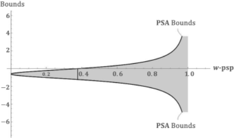
From Figure 2, for w-psp∈ [0.000, 0.377], Theorem 4 shows that the w-psp provides the bounds ([-1.228, 0.000] for w-psp= 0.377) on the total effect of the spray distance excluding the null, which implies that the spray distance must have a negative effect to improve the transfer efficiency. For w-psp> 0.377, since the bounds on the total effects include the null, it may be difficult to judge whether the total effect of the spray distance is positive or negative. Here, according to [Kuroki, 2008; Kuroki, 2012], the possibility of a positive total effect is excluded by expert knowledge.
4 Discussion
Inspired by the cosine similarity and the bias-variance tradeoff, we proposed a novel sensitivity analysis, the proportionbased sensitivity analysis of uncontrolled confounding bias in causal effects (PSA). Remarkably, (i) the PSA is formulated based on minimal causal knowledge, (ii) the PSA enables us to handle a set of covariates that consists of an uncertain number of discrete and continuous variables, (iii) the PSA can be interpreted as the proportion, and (iv) the PSP has an estimable cutoff value that prevents misleading causal judgment qualitatively through observed data. In particular, when we wish to know how the estimates of the average causal risk (causal risk difference) change when the value of the sensitivity parameters is changed since the PSA involves a single sensitivity parameter, it is easy to visualize the relationship between the average causal risk (causal risk difference) and the PSP in 2-D plots.
Acknowledgements
This research was partially supported by Grant-in-Aid for Scientific Research (C) from the Japan Society for the Promotion of Science, Grant Number 21H03504 and 24K14851.
@inproceedings{ijcai2024p789,
  title     = {Proportion-based Sensitivity Analysis of Uncontrolled Confounding Bias in Causal Inference},
  author    = {Yoshida, Haruka and Kuroki, Manabu},
  booktitle = {Proceedings of the Thirty-Third International Joint Conference on
               Artificial Intelligence, {IJCAI-24}},
  publisher = {International Joint Conferences on Artificial Intelligence Organization},
  editor    = {Kate Larson},
  pages     = {7136--7143},
  year      = {2024},
  month     = {8},
  note      = {Main Track},
  doi       = {10.24963/ijcai.2024/789},
  url       = {https://doi.org/10.24963/ijcai.2024/789},
}
TY - CPAPER TI - Proportion-based Sensitivity Analysis of Uncontrolled Confounding Bias in Causal Inference AU - Yoshida, Haruka AU - Kuroki, Manabu T2 - Proceedings of the Thirty-Third International Joint Conference on Artificial Intelligence, IJCAI-24 PB - International Joint Conferences on Artificial Intelligence Organization PY - 2024 SP - 7136 EP - 7143 DO - 10.24963/ijcai.2024/789 UR - https://doi.org/10.24963/ijcai.2024/789 ER -Copied
Machine-readable versions of this paper, for tools and AI agents:





