
Transfer Learning Using Inaccurate Physics Rule for Streamflow Prediction
Proceedings of the Thirty-Third International Joint Conference on Artificial Intelligence. AI for Good. Pages 7170-7178.
https://doi.org/10.24963/ijcai.2024/793
Keywords
- Data Mining: General
- Multidisciplinary Topics and Applications: General
Abstract
Accurate streamflow prediction is critical for ensuring water supply and detecting floods, while also providing essential hydrological inputs for other scientific models in fields such as climate and agriculture.
Recently, deep learning models have been shown to achieve state-of-the-art regionalization performance by building a global hydrologic model. These models predict streamflow given catchment physical characteristics and weather forcing data.
However, these models are only focused on gauged basins and cannot adapt to ungaugaed basins, i.e., basins without training data.
Prediction in Ungauged Basins (PUB) is considered one of the most important challenges in hydrology, as most basins in the United States and around the world have no observations.
In this work, we propose a meta-transfer learning approach by enhancing imperfect physics equations that facilitate model adaptation.
Intuitively, physical equations can often be used to regularize deep learning models to achieve robust regionalization performance under gauged scenarios, but they can be inaccurate due to the simplified representation of physics.
We correct such uncertainty in physical equation by residual approximation and let these corrected equations guide the model training process. We evaluated the proposed method for predicting daily streamflow on the catchment attributes and meteorology for large-sample studies (CAMELS) dataset.
The experiment results on hydrological data over 19 years demonstrate the effectiveness of the proposed method in ungauged scenarios.
- [Addor et al., 2017] Nans Addor, Andrew J Newman, Naoki Mizukami, and Martyn P Clark. The camels data set: catchment attributes and meteorology for large- sample studies. Hydrology and Earth System Sciences, 21(10):5293-5313, 2017.
- [Arnold et al., 2012] Jeffrey G Arnold, Daniel N Moriasi, Philip W Gassman, Karim C Abbaspour, Michael J White, Raghavan Srinivasan, Chinnasamy Santhi, RD Harmel, Ann Van Griensven, Michael W Van Liew, et al. Swat: Model use, calibration, and validation. Transactions of the ASABE, 55(4):1491-1508, 2012.
- [Bao et al., 2021] Tianshu Bao, Xiaowei Jia, Jacob Zwart, Jeffrey Sadler, Alison Appling, Samantha Oliver, and Tay- lor T Johnson. Partial differential equation driven dynamic graph networks for predicting stream water temperature. In 2021 IEEE International Conference on Data Mining (ICDM), pages 11-20. IEEE, 2021.
- [Bao et al., 2022] Tianshu Bao, Shengyu Chen, Taylor T Johnson, Peyman Givi, Shervin Sammak, and Xiaowei Jia. Physics guided neural networks for spatio-temporal super- resolution of turbulent flows. In Uncertainty in Artificial Intelligence, pages 118-128. PMLR, 2022.
- [Ben-David et al., 2010] Shai Ben-David, John Blitzer, Koby Crammer, Alex Kulesza, Fernando Pereira, and Jennifer Wortman Vaughan. A theory of learning from different domains. Machine learning, 79:151-175, 2010.
- [Besaw et al., 2010] Lance E Besaw, Donna M Rizzo, Paul R Bierman, and William R Hackett. Advances in un- gauged streamflow prediction using artificial neural net- works. Journal of Hydrology, 386(1-4):27-37, 2010.
- [Beven and Freer, 2001] Keith Beven and Jim Freer. Equi- finality, data assimilation, and uncertainty estimation in mechanistic modelling of complex environmental systems using the glue methodology. Journal of hydrology, 249(1- 4):11-29, 2001.
- [Blöschl and Sivapalan, 1995] Günter Blöschl and Mu- rugesu Sivapalan. Scale issues in hydrological modelling: a review. Hydrological processes, 9(3-4):251-290, 1995.
- [Blöschl et al., 2013] Günter Blöschl, Murugesu Sivapalan, Thorsten Wagener, Alberto Viglione, and Hubert Savenije. Runoff prediction in ungauged basins: synthesis across processes, places and scales. Cambridge University Press, 2013.
- [Both et al., 2021] Gert-Jan Both, Subham Choudhury, Pierre Sens, and Remy Kusters. Deepmod: Deep learning for model discovery in noisy data. Journal of Computational Physics, 428:109985, 2021.
- [Champion et al., 2019] Kathleen Champion, Bethany Lusch, J Nathan Kutz, and Steven L Brunton. Data- driven discovery of coordinates and governing equations. Proceedings of the National Academy of Sciences, 116(45):22445-22451, 2019.
- [Chen et al., 2021] Zeng Chen, Huan Xu, Peng Jiang, Sha- nen Yu, Guang Lin, Igor Bychkov, Alexey Hmelnov, Gen- nady Ruzhnikov, Ning Zhu, and Zhen Liu. A transfer learning-based lstm strategy for imputing large-scale con- secutive missing data and its application in a water qual- ity prediction system. Journal of Hydrology, 602:126573, 2021.
- [Chen et al., 2022a] Shengyu Chen, Jacob A Zwart, and Xi- aowei Jia. Physics-guided graph meta learning for pre- dicting water temperature and streamflow in stream net- works. In Proceedings of the 28th ACM SIGKDD Con- ference on Knowledge Discovery and Data Mining, pages 2752-2761, 2022.
- [Chen et al., 2022b] Shengyu Chen, Jacob A Zwart, and Xi- aowei Jia. Physics-guided graph meta learning for pre- dicting water temperature and streamflow in stream net- works. In Proceedings of the 28th ACM SIGKDD Con- ference on Knowledge Discovery and Data Mining, pages 2752-2761, 2022.
- [Chen et al., 2023] Shengyu Chen, Nasrin Kalanat, Yiqun Xie, Sheng Li, Jacob A Zwart, Jeffrey M Sadler, Alison P Appling, Samantha K Oliver, Jordan S Read, and Xiaowei Jia. Physics-guided machine learning from simulated data with different physical parameters. Knowledge and Infor- mation Systems, 65(8):3223-3250, 2023.
- [Dai et al., 2007] Wenyuan Dai, Qiang Yang, Gui-Rong Xue, and Yong Yu. Boosting for transfer learning.(2007), 193-200. In Proceedings of the 24th international confer- ence on Machine learning, 2007.
- [Feng et al., 2020] Dapeng Feng, Kuai Fang, and Chaopeng Shen. Enhancing streamflow forecast and extracting in- sights using long-short term memory networks with data integration at continental scales. Water Resources Re- search, 56(9):e2019WR026793, 2020.
- [Finn et al., 2017] Chelsea Finn, Pieter Abbeel, and Sergey Levine. Model-agnostic meta-learning for fast adaptation of deep networks. In International conference on machine learning, pages 1126-1135. PMLR, 2017.
- [Gauch et al., 2021] Martin Gauch, Frederik Kratzert, Daniel Klotz, Grey Nearing, Jimmy Lin, and Sepp Hochreiter. Rainfall-runoff prediction at multiple timescales with a single long short-term memory network. Hydrology and Earth System Sciences, 25(4):2045-2062, 2021.
- [He et al., 2024] Erhu He, Yiqun Xie, Licheng Liu, Zhenong Jin, Dajun Zhang, and Xiaowei Jia. Knowledge guided machine learning for extracting, preserving, and adapting physics-aware features. In Proceedings of the 2024 SIAM International Conference on Data Mining (SDM), pages 715-723. SIAM, 2024.
- [Hochreiter and Schmidhuber, 1997] Sepp Hochreiter and Jürgen Schmidhuber. Long short-term memory. Neural computation, 9(8):1735-1780, 1997.
- [Hsu et al., 1995] Kuo-lin Hsu, Hoshin Vijai Gupta, and Soroosh Sorooshian. Artificial neural network modeling of the rainfall-runoff process. Water resources research, 31(10):2517-2530, 1995.
- [Jia et al., 2019] Xiaowei Jia, Jared Willard, Anuj Karpatne, Jordan Read, Jacob Zwart, Michael Steinbach, and Vipin Kumar. Physics guided rnns for modeling dynamical sys- tems: A case study in simulating lake temperature profiles. In Proceedings of the 2019 SIAM International Confer- ence on Data Mining, pages 558-566. SIAM, 2019.
- [Jia et al., 2021a] Xiaowei Jia, Jared Willard, Anuj Karpatne, Jordan S Read, Jacob A Zwart, Michael Steinbach, and Vipin Kumar. Physics-guided machine learning for scientific discovery: An application in simu- lating lake temperature profiles. ACM/IMS Transactions on Data Science, 2(3):1-26, 2021.
- [Jia et al., 2021b] Xiaowei Jia, Yiqun Xie, Sheng Li, Shengyu Chen, Jacob Zwart, Jeffrey Sadler, Alison Ap- pling, Samantha Oliver, and Jordan Read. Physics-guided machine learning from simulation data: An application in modeling lake and river systems. In 2021 IEEE Interna- tional Conference on Data Mining (ICDM), pages 270- 279. IEEE, 2021.
- [Jia et al., 2021c] Xiaowei Jia, Jacob Zwart, Jeffrey Sadler, Alison Appling, Samantha Oliver, Steven Markstrom, Jared Willard, Shaoming Xu, Michael Steinbach, Jordan Read, et al. Physics-guided recurrent graph model for pre- dicting flow and temperature in river networks. In Pro- ceedings of the 2021 SIAM International Conference on Data Mining (SDM), pages 612-620. SIAM, 2021.
- [Jia et al., 2023] Xiaowei Jia, Shengyu Chen, Can Zheng, Yiqun Xie, Zhe Jiang, and Nasrin Kalanat. Physics- guided graph diffusion network for combining heteroge- neous simulated data: An application in predicting stream water temperature. In Proceedings of the 2023 SIAM Inter- national Conference on Data Mining (SDM), pages 361- 369. SIAM, 2023.
- [Karpatne et al., 2017] Anuj Karpatne, William Watkins, Jordan Read, and Vipin Kumar. Physics-guided neural net- works (pgnn): An application in lake temperature model- ing. arXiv preprint arXiv:1710.11431, 2017.
- [Kratzert et al., 2018] Frederik Kratzert, Daniel Klotz, Claire Brenner, Karsten Schulz, and Mathew Herrneg- ger. Rainfall-runoff modelling using long short-term<? xmltex\break?> memory (lstm) networks. Hydrology and Earth System Sciences, 22(11):6005-6022, 2018.
- [Kratzert et al., 2019] Frederik Kratzert, Daniel Klotz, Guy Shalev, Günter Klambauer, Sepp Hochreiter, and Grey Nearing. Towards learning universal, regional, and lo- cal hydrological behaviors via machine learning applied to large-sample datasets. Hydrology and Earth System Sci- ences, 23(12):5089-5110, 2019.
- [Li et al., 2022] Xiang Li, Ankush Khandelwal, Xiaowei Jia, Kelly Cutler, Rahul Ghosh, Arvind Renganathan, Shaom- ing Xu, Kshitij Tayal, John Nieber, Christopher Duffy, et al. Regionalization in a global hydrologic deep learn- ing model: from physical descriptors to random vectors. Water Resources Research, 58(8):e2021WR031794, 2022.
- [Neitsch et al., 2011] Susan L Neitsch, Jeffrey G Arnold, Jim R Kiniry, and Jimmy R Williams. Soil and water assessment tool theoretical documentation version 2009. Technical report, Texas Water Resources Institute, 2011.
- [Petersen et al., 2019] Brenden K Petersen, Mikel Landa- juela Larma, T Nathan Mundhenk, Claudio P Santi- ago, Soo K Kim, and Joanne T Kim. Deep symbolic regression: Recovering mathematical expressions from data via risk-seeking policy gradients. arXiv preprint arXiv:1912.04871, 2019.
- [Sadler et al., 2022] Jeffrey Michael Sadler, Alison Paige Appling, Jordan S Read, Samantha Kay Oliver, Xiaowei Jia, Jacob Aaron Zwart, and Vipin Kumar. Multi-task deep learning of daily streamflow and water temperature. Water Resources Research, 58(4):e2021WR030138, 2022.
- [Sahoo et al., 2018] Subham Sahoo, Christoph Lampert, and Georg Martius. Learning equations for extrapolation and control. In International Conference on Machine Learn- ing, pages 4442-4450. PMLR, 2018.
- [Sivapalan et al., 2003] Murugesu Sivapalan, K Takeuchi, SW Franks, VK Gupta, H Karambiri, V Lakshmi, X Liang, JJ McDonnell, EM Mendiondo, PE O'connell, et al. Iahs decade on predictions in ungauged basins (pub), 2003-2012: Shaping an exciting future for the hydrolog- ical sciences. Hydrological sciences journal, 48(6):857- 880, 2003.
References were extracted automatically from the PDF and may contain errors.
Full text extracted automatically from the PDF; figures, tables and equations may differ. The PDF is the version of record.
1 Introduction
Simulating hydrological processes is essential for modeling a variety of Earth science problems. In particular, accurate prediction of streamflow in river basins is important for simulating water cycles needed for a wide range of applications, including modeling of water quality, agriculture, climate, and greenhouse gas emissions. Besides, streamflow predictions
(b)
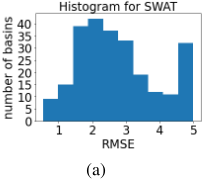
Figure 1: RMSE distribution by (a) the process-based SWAT model and (b) the global LSTM over all the basins. The rightmost bin in each figure represents the basins with RMSE ≥ 5.
are also essential for ensuring water supply while also providing early warnings of floods and droughts, which aids in a better management of aquatic ecosystems. The central challenge is about how to extrapolate to out-of-sample scenarios, e.g., predicting flows in ungauged basins, from instrumented to non-instrumented hillslopes, from areas with flux towers to areas without flux data, etc. [Blöschl and Sivapalan, 1995]. Often such extrapolation is achieved by using ancillary data (e.g. soil maps, remote sensing, digital elevation maps, etc.) to help understand similarities and differences between different areas. The regional modeling problem is thus closely related to the problem of prediction in ungauged basins [Blöschl et al., 2013; Sivapalan et al., 2003].
Traditionally, process-based models (also referred to as physical models) have been built for streamflow prediction, and they are often calibrated separately for each river basin. Most of these hydrological models are calibrated separately to each specific basin [Arnold et al., 2012]. The calibration process aims to derive hydrologic parameters for generating simulations that match available observations. This is challenging due to the strong interaction between individual model parameters (e.g., between soil porosity and soil depth, or between saturated conductivity and an infiltration rate parameter) [Beven and Freer, 2001], and requires substantial human labor and computational cost in the calibration process. Besides, most physics-based models are necessarily approximations of reality due to incomplete knowledge of certain processes or omission of processes to maintain computational efficiency.
Recently, there has been a growing interest in datadriven/machine learning (ML)-based streamflow modeling. Researchers have found that ML models benefit from learning jointly from a collection of different basins or locations because available observations are not sufficient for extracting complex water dynamics from a single basin [Kratzert et al., 2019; Chen et al., 2022a; Jia et al., 2021c]. Learning simultaneously from multiple basins requires the ML model to learn and encode the difference in basin characteristics so as to differentiate the hydrologic behaviors across basins. To better show the performance of ML models, we illustrate the comparison between the process-based SWAT model [Arnold et al., 2012] and ML model over a set of basins in the United States in Fig. 1. Despite the promise in predictive accuracy, ML methods remain limited in extrapolating to basins that are not included in the training set.
We propose a physics-guided meta-transfer learning approach that integrates data from multiple basins and adapts the model to capture the behaviors of each basin. The proposed meta-transfer learning approach aids in model adaptation to unseen basins by preserving the learned flow patterns, and thus ensure the generalization performance. Unlike traditional meta-learning approaches such as model-agnostic meta-learning (MAML) [Finn et al., 2017], we use a meta network to learn the parameters for estimating the model residual of each basin, which is then used to correct the streamflow prediction based on the physical equation. The main contribution of this work can be summarized as:
- We integrate a physical equation with the ML model, which reduces the size of parameters searching space and improves the model generalization.
- To address the imperfection of the physical equation, we use a lasso regression model to approximate the residual of physical simulations and mitigate the bias of the physical equation.
- We propose to use meta-learning to adapt the model to unlabeled tasks, i.e., unguaged basins. Specifically, we train a separate forward neural network to predict the lasso regression coefficients using static characteristics of each basin as its input.
- We enhance the physical equation using the approximated residual for both labeled and unlabeled datasets. Then we integrate the enhanced equation into the training process of the ML model.
- We also propose an alternative approach to iteratively update the simulated output from the enhanced physical equation and the predicted output from the ML model. The training process switches between the labeled and unlabeled datasets.
2 RelatedWork
Data-driven methods have been widely used to learn how to predict streamflow from weather drivers and catchment physical characteristics directly without involving any hydrological process [Kratzert et al., 2019; Li et al., 2022; Sadler et al., 2022]. Depending on whether one or multiple catchments of data are used, the data-driven model will learn localized or regionalized hydrological behaviors, respectively. A local model uses data from only one catchment. In contrast, a global model uses data from multiple catchments that encompass a wide range of available hydrological behaviors.
In particular, neural network-based models [Besaw et al., 2010; Hsu et al., 1995] are often used as the base model for data-driven approaches in hydrology. In recent years, the long short-term memory (LSTM) networks [Hochreiter and Schmidhuber, 1997], one subfamily of neural networks, has shown burgeoning applicability in streamflow prediction tasks [Kratzert et al., 2018]. For examples, [Kratzert et al., 2019] has shown that using physical characteristics will train a universal global LSTM-based model that outperforms process-based individual models given the same forcing data.
Process-based models of dynamical systems are traditional approaches used to study engineering [Bao et al., 2022] and environmental systems [Bao et al., 2021]. Despite their extensive use, these models have several well-known limitations due to incomplete or inaccurate representations of the physical processes being modeled. Given rapid data growth due to advances in sensor technologies, there is a tremendous opportunity to systematically advance modeling in these domains using ML methods.
One way to use ML approaches to enhance process-based models is through residual modeling. Residual is the difference between the output of a process-based model and the measured target variable. Thus, residuals capture the portion of the observed data that is not explained by the model. Several approaches can be used to explicitly represent the hidden information within the residual. For example, existing methods on symbolic regression [Petersen et al., 2019] and discovering equations [Champion et al., 2019; Both et al., 2021; Sahoo et al., 2018] provide alternative ways to find hidden equations from datasets. Symbolic regression outputs a combination of multiplication, division, addition, and subtraction of variables. This is similar to the lasso regression used in this work, except that we do not consider multiplication and division, as they are less interpretable. Also here we assume the residual has reduced complexity and thus do not consider differential terms in the residual equation.
3 ProblemDefinition
We consider N observed basins and M unobserved (or ungauged) basins in a region. For each basin i, we are provided with input features over T daily time step Xi = {x1i , x2i , ..., xTi }. Here input features xti form a Dx- dimensional vector, which includes dynamic weather drivers (e.g., air temperature, precipitation, evapotranspiration) and static characteristics of the basin (e.g., soil properties). Additionally, we have observed target variable (i.e., streamflow) Y = {yt i } for the observed basins on each date. Our objective is to predict streamflow over all the M ungauged basins at a daily scale by leveraging the contextual information and the knowledge learned from the gauged basins.
4 Methods
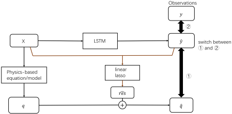
In this section, we formally describe our proposed method, as outlined in Figs. 2 and 3. We first introduce the LSTM model, which has been widely used for predicting streamflow in hydrology due to its ability to capture long-term temporal dependencies and preserve the temporal locality information of each data point [Feng et al., 2020; Gauch et al., 2021]. Then we discuss the regularization approach, which is further enhanced by the residual correction and input augmentation strategies to refine the LSTMmodel for different basins based on their physical characteristics. Finally, we develop an alternative training method to reduce the residual while having it guide the model training.
4.1 Preliminaries on LSTM
The recurrent neural network (RNN) model has been widely used to model temporal patterns in sequential data. The RNN model defines transition relationships for the extracted hidden representation through a recurrent cell structure. In this work, we adopt LSTM to build the recurrent layer for capturing long-term dependencies. LSTM is a special type of recurrent neural network, well suited for the task of rainfallrunoff, basin modeling, and most popular and widely used in hydrology for predicting streamflow [Chen et al., 2022b; Li et al., 2022]. The LSTM cell combines the input features xt at each time step and the inherited information from previous time steps. Here we omit the subscript i as we do not target a specific basin.
Each LSTM cell has a cell state ct , which serves as a memory and allows for preserving information from the past. Specifically, the LSTM first generates a candidate cell state ¯ct by combining xt and the hidden representation at the previous time step ht-1 , as follows:
where W and b are matrices and vectors, respectively, of learnable model parameters. Then the LSTM generates a forget gate f t , an input gate gt , and an output gate ot via sigmoid function σ(·), as follows:
The forget gate is used to filter the information inherited from ct-1 , and the input gate is used to filter the candidate cell state at t. Then we compute the new cell state as follows:
where ⊗ denotes the entry-wise product.
After obtaining the cell state, we can compute the hidden representation by filtering the cell state using the output gate, as follows:
According to the above equations, we can observe that the computation of ht combines the information at the current time step (xt ) and the previous time step (ht-1 and ct-1 ), and thus encodes the temporal patterns learned from the data.
In our problem, the final output ˆ yt is a linear transformation of ht . The regular loss function is defined as
where ˆ yt i represents the output of the neural networks at ith basin and tth day.
4.2 Regularization Using Physical Equations
According to the mass conservation law, the streamflow for each basin i can be simulated based on the information of rainfall, evapotranspiration, and change of soil water conditions, as follows:
where rainfallti represents daily average precipitation for basin i at time t, etti represents evapotranspiration, swti represents the soil water for basin i at time t, and qt i represents the streamflow simulated by the physical equation. In this work, we estimate the evapotranspiration and soil water condition using an uncalibrated physical model, SWAT [Neitsch et al., 2011; Arnold et al., 2012]. Due to the bias of the physical model in simulating these variables, we use the max operation on the right-hand side of Eq. 6 to ensure the simulated streamflow value is non-negative.
We consider the streamflow qt i simulated by the physical equation as pseudo labels. It is noteworthy that such pseudo labels can be generated for basins and periods without streamflow observations. We can modify the training objective (Eq. 5) by enforcing the consistency with physical laws via an additional physics-based regularization term. This can help mitigate model overfitting to the noisy measurement and stay consistent with the physical relationship [Jia et al., 2021a; Chen et al., 2023]. An additional benefit of adding the physics-based regularization term is that the computation of the regularization does not require real labels. Hence, instead of using the pseudo labels in the labeled dataset only, we also incorporate the pseudo labels in the unlabeled dataset (i.e., M ungauged basins). We can control the weight of regularization by a hyper-parameter λ. The updated training loss combines true observations yt i and the physics-based pseudo labels qt i as regularization, which is expressed as follows:
4.3 Residual Correction
One limitation of the regularization method is that the pseudo labels qt i obtained through Eq. 6 may be inaccurate due to bias of process-based models in estimating evapotranspiration and soil moisture. As a result, the regularization mechanism in Eq. 7 may negatively affect the model performance. To address this issue, we propose to refine the physical equation by separately predicting the residual between the pseudo label and the observed value, i.e., resti = qt i - yt i . If such residual can be modeled, we can use it to update the pseudo label and improve the regularization in Eq. 7.
To build such a residual-predicting model, we hypothesize that the residual depends on weather inputs, local watershed characteristics, and the current streamflow. Let resti be the output for the i basin at time t and sti = (xti , yt i ) be the input, which contains the feature vector x and the streamflow value. We use Lasso regression is to solve the following task:
where p is the dimension of input (i.e., Dx+1), βi is the constant coefficient for basin i, βi = (βi,1, βi,2, ..., βi,p) is the coefficient vector, and k is a prespecified free parameter that determines the degree of regularization. We run the Lasso regression over different basins separately, and each basin i has its own unique βi. This can help capture distinct hydrologic conditions across basins.
We emphasize that it is necessary to include the streamflow value yt i in the input sti in Eq. 8 due to the strong dependency between the residual and the streamflow variations. However, the true streamflow value is not accessible in unlabeled basins. So an initial guess for yt i (for i in 1 to M) in unlabeled basins is required. A straightforward way is to use the output of a basic LSTM as an approximation of yt i and treat it as the starting point.
Another challenge is that Lasso regression cannot be directly used for unlabeled basins due to the lack of observations needed to measure residuals resti . To enable the adaptation to ungaged basins, we build a forward neural network (FNN) to approximate the unknown βi. The input of the FNN is the static characteristics (included in xti ), which describe the distinctions amongst basins. The output of the FNN is the Lasso coefficients βi associated with the basin. This is essentially a meta-learning approach, as the obtained FNN model can learn a mapping from gauged basins that facilitates the residual prediction on target ungauged basins. The process is illustrated in Fig. 2.
4.4 Input Augmentation
Inspired by the prior work [Karpatne et al., 2017], we also augment the input features to the LSTMmodel with the corrected pseudo label. The augmented input feature vector for the LSTM is xtaug,i = (xti , qt i ). The intuition behind this is to combine the knowledge of physical model and neural network to overcome their complementary deficiencies and leverage information in both physics and data. In particular, the hybrid data model can learn to complement biases of physical model by extracting complex features from the space of neural network input, thus reducing our knowledge gaps. In labeled datasets, we denote
The enhanced pseudo label is calculated as
Algorithm 1 The proposed alternate training method
Initialize the LSTM and calculate qt i through (Eq. 6) for epoch = 1 : number of alternate epochs do for k = 1 : number of training iterations on q do for t = 1 : T, i = 1 : M do Make residual correction through (Eq. 9) end for Train the model using {ˆ qt i } through (Eq. 10) end for for l = 1 : number of training iterations on y do Train the model using {yt i } for t = 1 : T, i = 1 : N do Compute ˆ yt i and prepare the data for (Eq. 9) end for end for end for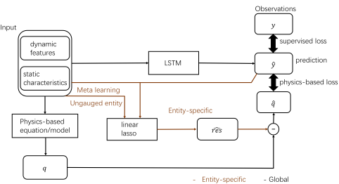
Then we can update the LSTM input as xtaug,i = (xti , ˆ qt i ). In unlabeled basins, we will approximate βi using the obtained FNN because we cannot run lasso regression in unlabeled datasets. Meanwhile, sti = (xti , yt i ) and yt i is missing, we use ˆ yt i from basic LSTM as an initial guess. Therefore, we get sti = (xti , ˆ yt i ) in unlabeled datasets, and then we calculate ˆ qt i (according to Eqs. 9 and 10) and update xtaug,i .
4.5 Alternate Training Between Pseudo Labels and True Observations
As an alternative to the regularization method, the pseudo labels obtained through the physical equation can be used to pre-train the ML model, which is then fine-tuned with observed labels [Jia et al., 2019; Jia et al., 2021a; Jia et al., 2023; Chen et al., 2023; Jia et al., 2021b]. The main concern with this approach is domain shifting [Ben-David et al., 2010], where fine-tuning in the target domain can distort the generalizable patterns learned by the pre-trained model, potentially causing overfitting [He et al., 2024]. To address this issue, we propose a new approach to alternately train the model on pseudo labels and true observations.
Specifically, we start training from corrected pseudo labels ˆ qt i obtained through Eq. 10, and then train the model on true observations. After that, we correct pseudo labels ˆ qt i using the updated predictions ˆ yt i and repeat this training process (Fig. 3).
5 Experiments
We evaluate the proposed method for predicting streamflow using the continental hydrology data set, CAMELS [Addor et al., 2017]. CAMELS encompasses a diverse set of basins across the contiguous US. In our experiments, we use 480 basins from the CAMELS dataset for evaluation. One-half of the basins are for training and the other half for testing. In the following, we will describe the datasets and baselines and also discuss the results of the predictive performance using the effectiveness of pretraining, residual correction, and model generalization. All experiments are conducted using TensorFlow on a computer with the following configuration: Intel Core i7-8750H CPU @2.20GHz × 6 Processor, 16 GiB Memory, GeForce GTX 1060, 64-bit Win10 OS. 1
5.1 Dataset and Baselines
Our experiments use the continental hydrology dataset, CAMELS. The CAMELS data set contains continuous meteorologic input, observed streamflow data, and catchmentdependent spatially varying but temporally static physical characteristics. CAMELS encompasses a total of 671 basins across the contiguous US. Due to some basin delineation errors [Addor et al., 2017], we followed the suggestion from [Kratzert et al., 2019] to select 480 basins whose boundaries are confirmed to be correctly delineated without digital errors. Each basin is supplied with observed discharge and climate-forcing data from remote sensing products, climate models, and data assimilation with daily temporal resolution. Additionally, a corresponding hydrological model (SAC-SMA, Sacramento Soil Moisture Accounting model) is well-calibrated for each basin and its physical simulation is also available. Adopting such a wide distribution of basins, CAMELS provides a comprehensive and detailed physical description of basins. Selecting only a subset of those features as suggested by [Kratzert et al., 2019], we choose 27 physical descriptors from climatology, geomorphology, and geology perspectives to characterize and discriminate across basins. The data period starts on 10/2/1989 and ends on 9/29/2008. We use the odd index basins for training and even index basins for testing. We set the learning rate to 0.001 and update the model for 50 epochs. Descriptions of the baselines are provided below.
1 Code for the experiment is available at drive.google.com/drive/folders/1umw7gAdfVnPEH_ALn4gnAR1 j_3czFd2i?usp=sharing
Pre-Train + Fine-Tuning
We pretrain the LSTM model on all pseudo labels and then train it on true labels. The pre-training process takes 50 epochs.
Alternate Training Between Pseudo Labels and True Observations
As described in Section 4.5, we train the model with the pseudo labels for a few iterations, and then tune the model with true labels. We repeat this alternate training process for a few times.
Perturbation to the Proposed Methods
To test the robustness of our approaches, we perturb the evaporation and soil water data in Eq. 8 and test the model's performance and robustness.
LSTM + Tradaboost
This is a transfer learning baseline [Chen et al., 2021] with the aim of transferring the knowledge from simulated data to real data. It integrates LSTMwith instance-based transfer learning through tradaboost [Dai et al., 2007]. Tradaboost extends boosting-based learning algorithms and allows utilizing a small amount of newly labeled data to leverage the old data to construct a high-quality model for the new data.
5.2 Performance Evaluation
We report the testing performance of different methods for streamflow prediction in the tables. We also test the performance of each model using less training data. In particular, we randomly select 60 and 120 labeled basins from the 240 labeled basins for training the model. We repeat each experiment five times with random model initialization and report the mean of the rooted mean square error (RMSE). Next, we discuss the results from several different aspects.
Pre-Train + Fine-Tuning
The pre-train-fine-tune method is widely used in many ML applications. As shown in Table 1, the model can achieve the best performance with less fine-tuning epochs. For fine-tuning with fewer data (60 basins), we can adopt the pre-trained model directly to avoid overfitting to this small dataset. When we are given more training data (120, 240 basins), the model can better learn flow dynamics through more fine-tuning epochs. For 120 basins, the model achieves the best performance when fine-tuned with 10 epochs. Compared with the previous case (60 training basins), the model needs more fine-tuning epochs to learn the useful information from the training set. For 240 basins, the model performs the best with more fine-tuning epochs (30 epochs). Here the target domain (true labels) is of the same size as the source domain (pseudo labels), and thus it is worth training more epochs on the target domain. However, one major concern is that we cannot decide the best number of fine-tuning epochs before the training. The obtained trend shows that one may want to fine-tune more epochs in general for large datasets. A separate validation set can also be used to address this issue.
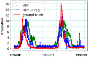
- (a) LSTM vs. LSTM + regularization
- (d) pretrain + fine tuning vs. alternate training on pseudo labels and true labels
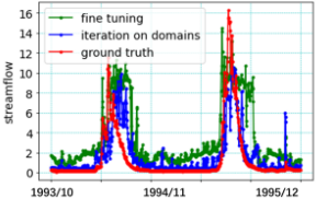
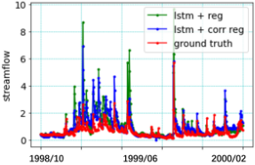
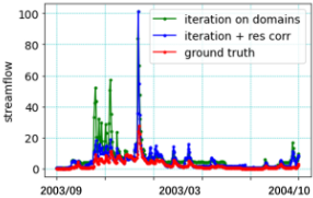
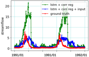
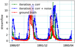
Figure 4: Streamflow predictions using different methods. Figure 4(a) is in basin 462. Figure 4(b) is in basin 214. Figure 4(c) is in basin 472. Figure 4(d) is in basin 462. Figure 4(e) is in basin 492. Figure 4(f) is in basin 462.
General Performance for All Methods
Table 2 summarizes the general performance of all methods considered in our test. For the regularization-based methods, the performance is quite similar with the alternate training methods on large datasets, but becomes much worse on small datasets. This is because the regularization methods do not utilize the entire set of pseudo labels, thus making the actual training datasets very small. Meanwhile, with large datasets, the regularization methods can even outperform some alternate training methods due to the augmented physics input. The output of physical model and original features can overcome their complementary deficiencies and leverage information in both the physical model and observation data. The fine-tuning-based methods are more stable on small datasets and outperform regularization methods significantly, but they can suffer from the domain shifting. The tradaboost + LSTM method achieves accurate predictions on small datasets but performs poorly on large datasets.
Regularization-Based Methods
Table 3 summarizes the performance of all the regularization methods. It can be seen that the basic LSTM performs the worst. The standard regularization can help LSTM stay consistent with the pseudo label, resulting in slight improvement in predictive accuracy.
We also use regularization on all pseudo labels (including unlabeled basins) to further handle data insufficiency. With 60 basins of labeled data, the result of regularization-based method is quite similar to the pretraining methods, both of which use global patterns learned from all the basins. As we increase the size of training datasets, the predictions get worse. It is because the regularization could disrupt the true underlying patterns that can be learned from observations.
In order to improve the efficiency of regularization, we add the residual correction method to refine the pseudo labels. The RMSE gets reduced in every aspect on various training datasets. Furthermore, we add the corrected pseudo labels to the model input instead of using them in the regularization solely, and thus further improve our results. Regularization + physics input + residual correction model provides the best results we can obtain across all the methods.
Alternate Training Methods
Besides the regularization methods, we also utilize the alternate training methods to prevent overfitting. In Table 4, we compare the 3 methods mentioned above. The plain pretrain + fine-tuning model overfits small datasets but achieves an average performance as the basic LSTM model on the full dataset. The alternate training methods can mitigate overfitting by switching training domains and preserving the existing patterns in the pseudo-label domain. Finally, our proposed method (iteration + residual correction) can make an even better prediction on small datasets (60, 120 basins), which is the best performance that can be achieved across all the methods. The improvement is smaller when using the full training dataset because the corrected pseudo labels do not play a significant role given sufficient real labels.
| basins | 0 ep | 10 eps | 20 eps | 30 eps | 40 eps |
|---|---|---|---|---|---|
| 60 | 2.316 | 2.535 | 2.751 | 3.234 | 2.878 |
| 120 | 2.357 | 2.105 | 2.206 | 2.651 | 2.562 |
| 240 | 2.245 | 2.013 | 2.020 | 1.945 | 2.137 |
| Method | 60 bs | 120 bs | 240 bs |
|---|---|---|---|
| basic LSTM | 11.871 | 9.384 | 2.082 |
| LSTM+ regularization | 10.923 | 9.036 | 2.005 |
| pretrain + fine-tuning | 4.164 | 3.037 | 2.092 |
| LSTM + tradaboost | 2.688 | 2.587 | 2.302 |
| LSTM+ reg + phy + corr | 7.316 | 6.449 | 1.937 |
| iteration on domains | 2.194 | 2.168 | 1.995 |
| iteration + correction | 2.116 | 2.133 | 1.966 |
| Method | 60 bs | 120 bs | 240 bs |
|---|---|---|---|
| basic LSTM | 11.871 | 9.384 | 2.082 |
| LSTM+ regularization | 10.923 | 9.036 | 2.005 |
| LSTM + reg (all data) | 3.011 | 3.130 | 3.236 |
| LSTM + reg + corr | 9.527 | 7.703 | 1.962 |
| LSTM+ reg + phy + corr | 7.316 | 6.449 | 1.937 |
Robustness of the Alternate Training Method
Table 5 summarizes the model robustness and performance under noise perturbation. We add 0.02 standard deviation error to the evapotranspiration and soil water data to test the robustness of the proposed method. The traditional alternate training method between pseudo labels and true labels does not show strong robustness to perturbation, and there is an obvious RMSE increase. However, our proposed method (iteration + residual correction) shows strong stability in handling noisy data due to the residual correction. The effect of added noise has been canceled during the residual correction process.
Ablation Study
Figs. 5(a), 5(b), 5(c) and 5(d) show the ablation study between different methods. Each dot represents a single test basin and the values in x-y axis denote RMSE. The performance varies over different basins and most of the basins concentrate on left down corner.
6 Conclusion
In this paper, we propose two methods to handle transfer learning by leveraging inaccurate physics equations. We apply the proposed methods to streamflow prediction using realworld data over a diverse set of basins. To deal with the imperfection of physical equations, we use a Lasso regression to correct the residual caused by the rule and then let them rejoin the training process. Our methods show strong resistance to data absence and noise interference and a predictive performance comparable to that of the model using actual physical descriptors.
| Method | 60 basins | 120 basins | 240 basins |
|---|---|---|---|
| pretrain + fine-tuning | 4.164 | 3.037 | 2.092 |
| iteration on domains | 2.194 | 2.168 | 1.995 |
| iteration + correction | 2.116 | 2.133 | 1.966 |
| Method | 60 basins | 120 basins | 240 basins |
|---|---|---|---|
| iteration on domains | 2.194 | 2.168 | 1.995 |
| iteration + noise | 2.361 | 2.192 | 2.018 |
| iteration + corr + noise | 2.296 | 2.144 | 1.949 |
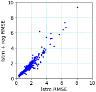
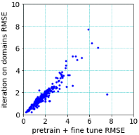
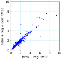
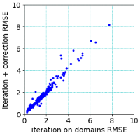
Figure 5: Ablation study for all methods.
Future work will include the improvement of the approximation of the physical equation while ensuring that it can be adapted to ungaged basins. We may also explore advanced ML models, such as Transformer-based models and other types of temporal neural network models, to further improve our streamflow prediction.
Acknowledgements
This research is funded by NSF grants 2028001, 2147195, 2239175, 2316305, and USGS grant No. G21AC10207.
@inproceedings{ijcai2024p793,
  title     = {Transfer Learning Using Inaccurate Physics Rule for Streamflow Prediction},
  author    = {Bao, Tianshu and Johnson, Taylor Thomas and Jia, Xiaowei},
  booktitle = {Proceedings of the Thirty-Third International Joint Conference on
               Artificial Intelligence, {IJCAI-24}},
  publisher = {International Joint Conferences on Artificial Intelligence Organization},
  editor    = {Kate Larson},
  pages     = {7170--7178},
  year      = {2024},
  month     = {8},
  note      = {AI for Good},
  doi       = {10.24963/ijcai.2024/793},
  url       = {https://doi.org/10.24963/ijcai.2024/793},
}
TY - CPAPER TI - Transfer Learning Using Inaccurate Physics Rule for Streamflow Prediction AU - Bao, Tianshu AU - Johnson, Taylor Thomas AU - Jia, Xiaowei T2 - Proceedings of the Thirty-Third International Joint Conference on Artificial Intelligence, IJCAI-24 PB - International Joint Conferences on Artificial Intelligence Organization PY - 2024 SP - 7170 EP - 7178 DO - 10.24963/ijcai.2024/793 UR - https://doi.org/10.24963/ijcai.2024/793 ER -Copied
Machine-readable versions of this paper, for tools and AI agents:





