
Predicting Housing Transaction with Common Covariance GNNs
Proceedings of the Thirty-Third International Joint Conference on Artificial Intelligence. AI for Good. Pages 7323-7330.
https://doi.org/10.24963/ijcai.2024/810
Keywords
- Machine Learning: General
- Multidisciplinary Topics and Applications: General
Abstract
Urban migration is a significant aspect of a city's economy. The exploration of the underlying determinants of housing purchases among current residents contributes to the study of future trends in urban migration, enabling governments to formulate appropriate policies to guide future economic growth. This article employs a factor model to analyze data on residents' rentals, first-time home purchases, and subsequent housing upgrades. We decompose the factors influencing housing purchases into common drivers and specific drivers. Our hypothesis is that common drivers reflect universal social patterns, while personalized drivers represent stochastic elements. We construct a correlation matrix capturing the inter-resident relationships based on the common drivers of housing purchases. We then propose a graph neural network based on the correlation matrix to model housing predictions as a node classification problem. Our model addresses two critical questions. Firstly, we aim to identify which part of rental residents will engage in first-time home purchases in the future. Secondly, we seek to determine which group of residents, having completed rental and first-time home purchases, will opt for a second home purchase. The results of our testing on real-world datasets demonstrate that based solely on rental and home purchase records, we can achieve a sensitivity for housing predictions exceeding 80%.
- [Bikmetova et al., 2023] Natalya Bikmetova, Geoffrey K Turnbull, and Velma Zahirovic-Herbert. Ethnicity in hous- ing markets: Buyers, sellers and agents. Real Estate Eco- nomics, 51(1):196-232, 2023.
- [Bourassa et al., 2007] Steven C Bourassa, Eva Cantoni, and Martin Hoesli. Spatial dependence, housing submarkets, and house price prediction. The Journal of Real Estate Finance and Economics, 35:143-160, 2007.
- [Defferrard et al., 2016] Michaël Defferrard, Xavier Bres- son, and Pierre Vandergheynst. Convolutional neural networks on graphs with fast localized spectral filtering. In Proceedings of the 30th International Conference on Neural Information Processing Systems, NIPS'16, pages 3844-3852, Red Hook, NY, USA, 2016.
- [Du et al., 2017] Jian Du, Shanghang Zhang, Guanhang Wu, José MF Moura, and Soummya Kar. Topology adaptive graph convolutional networks. arXiv preprint arXiv:1710.10370, 2017.
- [Gilbukh et al., 2023] Sonia Gilbukh, Andrew Haughwout, Rebecca J Landau, and Joseph Tracy. The price-to-rent ratio: A macroprudential application. Real Estate Eco- nomics, 51(2):503-532, 2023.
- [Gilmer et al., 2017] Justin Gilmer, Samuel S Schoenholz, Patrick F Riley, Oriol Vinyals, and George E Dahl. Neu- ral message passing for quantum chemistry. In Interna- tional conference on machine learning, pages 1263-1272.
- PMLR, 2017.
- [Hamilton et al., 2017] William L. Hamilton, Rex Ying, and Jure Leskovec. Inductive representation learning on large graphs. In Proceedings of the 31st International Confer- ence on Neural Information Processing Systems, NIPS'17, pages 1025-1035, Red Hook, NY, USA, 2017.
- [Hu et al., 2023] Mingzhi Hu, Zhenguo Lin, and Yingchun Liu. Amenities, housing affordability, and education elites. The Journal of Real Estate Finance and Economics, 66(1):141-168, 2023.
- [Kipf and Welling, 2017] Thomas N. Kipf and Max Welling. Semi-supervised classification with graph convolutional networks. In Proceedings of the Fifth International Con- ference on Learning Representations, ICLR 2017, 2017.
- [Koeniger et al., 2022] Winfried Koeniger, Benedikt Lennartz, and Marc-Antoine Ramelet. On the transmis- sion of monetary policy to the housing market. European Economic Review, 145:104107, 2022.
- [Kumar, 2019] Adarsh Kumar. House rent price prediction. International Research Journal of Engineering and Tech- nology, 6(04):3188-3191, 2019.
- [Liu et al., 2023] Bin Liu, Jiujun He, Ziyuan Li, Xiaoyang Huang, Xiang Zhang, and Guosheng Yin. Interpret esg rating's impact on the industrial chain using graph neural networks. In Proceedings of the Thirty-Second Interna- tional Joint Conference on Artificial Intelligence, IJCAI- 23, pages 6076-6084, 8 2023. AI for Good. IJCAI
- [Madhuri et al., 2019] CH. Raga Madhuri, G. Anuradha, and M. Vani Pujitha. House price prediction using regres- sion techniques: A comparative study. In 2019 Interna- tional Conference on Smart Structures and Systems (IC- SSS), pages 1-5, 2019.
- [Ming et al., 2020] Yue Ming, Jie Zhang, Jiaming Qi, Tian Liao, Maolin Wang, and Lingli Zhang. Prediction and analysis of chengdu housing rent based on xgboost algo- rithm. In Proceedings of the 3rd International Conference on Big Data Technologies, pages 1-5, 2020.
- [Miyakawa et al., 2022] Daisuke Miyakawa, Chihiro Shimizu, and Iichiro Uesugi. Do foreign buyers pay more than domestic buyers? evidence from international transaction-level data. The Journal of Real Estate Finance and Economics, pages 1-31, 2022.
- [Park and Bae, 2015] Byeonghwa Park and Jae Kwon Bae. Using machine learning algorithms for housing price pre- diction: The case of fairfax county, virginia housing data. Expert systems with applications, 42(6):2928-2934, 2015.
- [Price, 1993] Barbara Price. A first course in factor analysis. Technometrics, 35:453-453, 1993.
- [Seya and Shiroi, 2022] Hajime Seya and Daiki Shiroi. A comparison of residential apartment rent price predictions using a large data set: Kriging versus deep neural network. Geographical Analysis, 54(2):239-260, 2022.
- [Sihag et al., 2022] Saurabh Sihag, Gonzalo Mateos, Corey McMillan, and Alejandro Ribeiro. covariance neural net- works. In S. Koyejo, S. Mohamed, A. Agarwal, D. Bel- grave, K. Cho, and A. Oh, editors, Advances in Neural In- formation Processing Systems, volume 35, pages 17003- 17016.
- Curran Associates, Inc., 2022.
- [Varma et al., 2018] Ayush Varma, Abhijit Sarma, Sagar Doshi, and Rohini Nair. House price prediction using ma- chine learning and neural networks. In 2018 Second In- ternational Conference on Inventive Communication and Computational Technologies (ICICCT), pages 1936-1939, 2018.
- [Veličković et al., 2018] Petar Veličković, Guillem Cucurull, Arantxa Casanova, Adriana Romero, Pietro Liò, and Yoshua Bengio. Graph attention networks. In Interna- tional Conference on Learning Representations, 2018.
- [Wong et al., 2022] Siu Kei Wong, Kuang Kuang Deng, and Ka Shing Cheung. Starter home premium and housing af- fordability. The Journal of Real Estate Finance and Eco- nomics, pages 1-22, 2022.
- [Yoshida et al., 2022] Takahiro Yoshida, Daisuke Mu- rakami, and Hajime Seya. Spatial prediction of apartment rent using regression-based and machine learning-based approaches with a large dataset. The Journal of Real Estate Finance and Economics, pages 1-28, 2022.
- [Zhang et al., 2024] Yanjiang Zhang, Yong Tu, and Yongheng Deng. Duration-dependent transaction tax effects on sellers and their behaviors. Real Estate Economics, 52(1):140-183, 2024.
References were extracted automatically from the PDF and may contain errors.
Full text extracted automatically from the PDF; figures, tables and equations may differ. The PDF is the version of record.
1 Introduction
In China, the real consumer groups for renting and purchasing houses are the post-80s and post-90s generations. When young graduates choose to work in a particular city after completing their university education, their first challenge is finding rental accommodation. Some individuals realize that staying in the city benefits their career development, or they consider factors such as the city's infrastructure, leading them to choose to purchase a property and settle down in that city. As they age and their income increases, they may opt to upgrade to a more comfortable house to meet the needs of marriage and raising children. We consider these factors to be common drivers for housing purchases. Individuals influenced by this factor form a typical group that follows the trajectory of renting, purchasing for the first time, and subsequently upgrading their housing. The number of individuals in this group and their life trajectories validate the extent to which they integrate into the city. Therefore, studying the driving forces behind the growth of this group from renting to first-time purchases and subsequent upgrades holds significant implications for the future development of cities.
∗Corresponding author: liubin@swufe.edu.cn
Existing literature on real estate economics primarily focuses on studying either the behavior of renting alone [Kumar, 2019; Ming et al., 2020; Seya and Shiroi, 2022; Yoshida et al., 2022] or the behavior of purchasing alone [Park and Bae, 2015; Madhuri et al., 2019; Varma et al., 2018], while neglecting the continuous evolution from renting to purchasing and subsequent upgrades, as well as the driving factors behind them. These studies typically employ traditional statistical models such as ridge regression, LASSO, tree models, and vector autoregressive to analyze housing prices directly [Madhuri et al., 2019; Park and Bae, 2015; Ming et al., 2020; Yoshida et al., 2022]. Some studies utilize neural networks, such as LSTM [Varma et al., 2018]. However, these studies lack an exploration of the interrelationships among home buyers.
Other studies, although examining housing characteristics and social characteristics of homebuyers, such as the educational level of buyers [Hu et al., 2023], ethnic groups of buyers [Bikmetova et al., 2023; Miyakawa et al., 2022], and the infrastructure of the city where the houses are located [Hu et al., 2023], approach their research from the perspective of renting or purchasing individually.
This paper investigates the processes of renting, first-time purchases, and subsequent upgrades together, attempting to identify common and universal driving factors behind group housing behaviors while excluding personalized factors. We believe that capturing common factors will facilitate accurate predictions of future housing transactions, while personalized factors represent stochastic elements that are difficult to predict. For instance, individuals who are prepared to buy a home, driven by factors such as the desire to establish roots in their current city following career advancement, share similar motivations with those who are not yet ready to make a purchase due to intentions of relocating or limited financial capacity. These shared motivations, whether for purchasing or refraining from purchasing, form the fundamental factors in the construction of a resident graph. In contrast, personal factors usually represent randomness and they are difficult to predict. For example, certain individuals may be drawn to houses with peculiar or avant-garde architectural designs, considering them as conversation starters or artistic expressions.
Based on rental and purchase records, we employ a factor model to model the common factors driving residents' housing purchases and upgrades. Furthermore, through covariance analysis based on the factor model, we remove the covariance of personalized residuals in the sample covariance matrix of rental and purchase records, retaining only the covariance of common factors. The covariance of common factors among residents characterizes their correlation in terms of common housing purchasing drivers. Based on the derived correlation of underlying common housing purchasing drivers, we construct a graph G = (V, E) representing the relationships among residents, where nodes V represent residents and edges E represent the similarity of housing purchasing drivers between residents. It is important to note that the presence of edges connecting residents in E does not necessarily imply the existence of a social relationship between them. Subsequently, using the graph G, we employ a graph neural network [Gilmer et al., 2017; Kipf and Welling, 2017; Liu et al., 2023] to model housing predictions as a node classification problem. Finally, we validate our algorithm on a dataset of rental and purchase records. Compared to traditional models such as logistic regression and tree models, the graph neural network, which considers the correlation of residents' housing intentions, better leverages the information within the data and achieves superior predictive results.
Our contributions can be summarized as follows: 1) First, we use a factor model to model the common factors underlying housing purchases. 2) Second, We employ a graph neural network to model housing behavior as a node classification problem. 3) Finally, we study the above issues from the perspective of the entire process of renting, purchasing, and upgrading, and validate our approach on real-world data.
2 RelatedWorks
2.1 Price Prediction
Most existing literature on house price or rent price forecasting is macro analysis [Ming et al., 2020; Seya and Shiroi, 2022; Gilbukh et al., 2023], and a large portion of them prefer to use statistical [Yoshida et al., 2022; Bourassa et al., 2007] and machine learning methods [Madhuri et al., 2019; Varma et al., 2018]. Madhuri et al. [2019] use various machine learning methods including Ridge, LASSO, Elastic Net, boosting, etc., to predict the reasonable prices of houses and when these prices will occur. Varma et al. [2018] weights the various machine learning techniques and proposes to use real-time neighborhood details using Google Maps to get exact real-world valuations. In addition to helping buyers and sellers, better-estimated prices also guide financial institutions to better real estate appraisals [Park and Bae, 2015].
From a macro perspective, factors like location, housing area, transportation, and infrastructure are incorporated into features and fitted by machine learning models [Kumar, 2019]. Seya and Shiroi [2022] further perform rent price prediction on a large dataset and introduces deep neural networks to enhance the accuracy. These forecasts combine a variety of machine learning methods and are made from the perspectives of different stakeholders. Guidance is massively provided on macro price adjustments and home-buying policies.
2.2 Home-buying Behavior Studies
Residents' decisions regarding home purchases, however, are not solely dictated by housing prices. Their inclination to buy houses is also influenced by the dynamics of the rental market [Koeniger et al., 2022]. In times of economic downturn, purchasing a house through a mortgage entails an escalated level of risk. Moreover, the presence of capital constraints can serve as a significant impediment, hindering cash-poor households from realizing their goal of owning a property [Wong et al., 2022]. When considering the intention to purchase a house, which encompasses factors such as housing affordability, Hu et al. [2023] investigates the amenity conditions of cities as a means to analyze the appeal of cities to elite talent. The study explores this phenomenon by examining various aspects of cities. Furthermore, Miyakawa et al. [2022] compare the effects of educational attainment and domestication on the outcomes related to responses to housing requirements and housing premiums, respectively. These studies analyze the influence of these factors on individuals' reactions to housing-related aspects.
The above studies analyze only one or two of the selected aspects influencing home-buying behaviors [Zhang et al., 2024; Bikmetova et al., 2023]. Most of them only consider the influence of the external environment on people's decision-making and market transformation, ignoring the characteristics of people themselves [Ming et al., 2020; Seya and Shiroi, 2022; Gilbukh et al., 2023; Yoshida et al., 2022; Bourassa et al., 2007; Madhuri et al., 2019; Miyakawa et al., 2022]. Therefore, they are unable to combine macro changes and individual characteristics together to make predictions about specific residents.
3 Background and Dataset
The data utilized in this paper comprises micro-data from lease contracts, new commercial housing transactions, and stock housing sales contracts in a provincial capital city. Two distinct datasets are collected for analysis: a dataset pertaining to first-time home purchases and another dataset focusing on subsequent housing upgrades, {Xi , yi } ∈ Rni×pi , yi ∈ {1, 0}ni are the labels, i ∈ {1, 2}, where ni is the number of samples and pi is the dimension of the feature.
The first dataset, denoted as X1 , y1 , consists of rental data paired with first home-purchase records. It comprises a total of n1 = 25, 000 individual samples. Each sample is characterized by ten variables, which include four categorical variables (XB, RentType, In Province, In City) and six numerical variables (FWMJ, CZMJ, YZJ, Age, RenterAge, MonthlyRentUnitArea). Therefore, the dimensionality of this dataset is p1 = 10.
| Index | Feature Name | Meaning(Full Name) |
|---|---|---|
| 1 | XB | Gender |
| 2 | FWMJ | Area of the Rental House |
| 3 | FWMJ.1 | Area of the House Bought |
| 4 | CZMJ | Actual Living Area of Tenants in the Rental House |
| 5 | YZJ | Monthly Rent |
| 6 | FWZJ | Total Price of the House Bought |
| 7 | Age | Age |
| 8 | RentType | Whole Lease or not |
| 9 | RenterAge | Age of the Resident at the Time of Rental |
| 10 | BuyerAge | Age of the Resident at the Time of the Purchase |
| 11 | MonthlyRentUnitArea | Monthly Rent Required to Rent An Unit Area |
| 12 | SFAJ | Mortgage or not |
| 13 | In Province | Native of the Province or not |
| 14 | In City | Native of the City or not |
The second dataset, denoted as X2 , y2 , is designed to predict the likelihood of purchasing a second house based on rental and first-time home purchase records. This dataset comprises n2 = 13, 000 samples, with each sample containing thirteen characteristics (p2 = 13). These characteristics consist of five categorical variables (XB, RentType, SFAJ, In Province, In City) and eight numerical variables (FWMJ, FWMJ.1, CZMJ, FWZJ, YZJ, Age, BuyerAge, MonthlyRentUnitArea). For a comprehensive understanding of the features, please refer to Table 1, which provides detailed definitions and interpretations.
4 Methodology
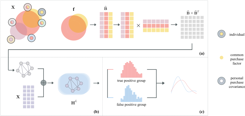
In this section, we begin by presenting the methodology for constructing a resident-resident correlated graph using their shared covariance in housing purchases. Subsequently, we provide a comprehensive review of the development of graph neural networks (GNNs) and then introduce our proposed approach, which builds upon these advancements. The overall architecture is as shown in Figure 1.
4.1 Graph Construction with a Factor Model
We think that residents are interconnected due to their shared underlying motivations for home purchasing. In light of this, we propose constructing a graph G to represent these common connections.
Our dataset can be represented as X, y, where X = (x1, · · · , xp) ∈ Rn×p denotes the feature matrix. Here, n corresponds to the number of observations, and p represents the dimension of each record. The labels for home purchase are denoted by y ∈ {1, 0}n , where the value 1 indicates a purchase, and 0 indicates no purchase. The resident's relationship can be captured by the sample covariance matrix,
which is computed using all the features, encompassing both the common and individual factors. In this study, our objective is to eliminate the individual factors and exclusively retain the common-shared factors for constructing the residentresident graph. To accomplish this, we employ a factor model to decompose the covariance matrix into two distinct components. Specifically, for each record xi, we have
where B = (b1, · · · , bm)⊤ ∈ Rp×k is the factor loading matrix, and bi = (bi1, · · · , bim)⊤, where i = 1, · · · , p. f = (f1, · · · , fm)⊤ are the common factors as we stated before, ϵ = (ϵ1, · · · , ϵp) are p idiosyncratic errors uncorrelated the factors f . We assume that E[ϵ|f] = 0, and Cov(ϵ|f ) = diag(σ2 1 , · · · , σ2 p ).
According to Eq.2, the Covariance matrix Σ of X can be decomposed as,
that is Σ contains two parts, the second part Cov(ϵ|f ) are resident specific covariance, and the first part BCov(f)B⊤ are the covariance of the common factors. In this work, we prefer to use the first part covariance BCov(f)B⊤ to construct resident-resident relationships based on the common driver of home-purchase.
In practice, we usually assume that the common factors are uncorrelated with one another, it suggests that Cov(fi, fj) = 0, i ̸= j, Var(fi) = 1, i, j = 1, · · · ,m, that is Cov(f) = I. Hence, the resident-resident correlated matrix can be simplified as BB⊤. The factor loading matrix B can be easily estimated by a spectral decomposition of the sample covariance ̂Σ [Price, 1993],
4.2 Graph Neural Networks
G = (V, E) is a graph with n nodes, where V = {1, . . . , n} is the set of n nodes and E ⊆ V ×V is the set of edges connecting paired residents in V. Let A = {aij}ni,j=1 denotes n × n symmetric adjacency matrix, where aij = 1 if there exists an edge eij ∈ E between nodes i and j, and aij = 0 otherwise. And X ∈ Rn×p denotes the feature matrix of the n nodes. With these notations, we revisit the classical GNNs within the framework of message-passing neural networks (MPNNs) [Gilmer et al., 2017], which involve three essential steps: neighbor set defining, followed by feature aggregation, and feature updating as the third step.
GraphConvolutional Network (GCN) [Kipf andWelling, 2017] The basic building block of a GCN is the graph convolutional layer, which operates on the node features and their connections in a graph,
where g(·) is a function return neighbors for node i, Hl-1 = (hl-1 1 , · · · , hl-1 n ) are the hidden node embeddings of (l-1)- layer, H0 = X, Aggre(·) and Com(·) are the feature aggregation and state update functions respectively. Wl are the parameters of the update function of layer l, L is the number of layers.
GraphSage GraphSage [Hamilton et al., 2017] learns node representations in large-scale graphs by sampling s local neighbors,
GraphSage extends the GCN neighbor set, where s ∈ N+.
Graph Attention Network (GATs) [Veliˇckovi´c et al., 2018] GATs assign different attention weights to neighboring nodes during the message-passing process, allowing the network to selectively aggregate the most relevant nodes for each target node,
GATs extend the GCN neighbor index function as g : S+ × Rn×dl-1 -→ {(j, αij)|aij = 1}, where αij is a attention weight between node i and its neighbor j.
VNN Sihag et al. [2022] proposed Covariance Neural Networks (VNN), wherein the adjacent matrix A in Eq. (5) is replaced by the sample covariance matrix ̂Σ (Eq. (1)). Additionally, they incorporate its m-order polynomial ∑mk=1 βk ̂Σk . Thus, the modified expression can be represented as follows:
where g : S+ -→ {j|[∑mk=1 βk ̂Σk ]ij ̸= 0} is a general neighbor index function. VNN can be considered as an equivalent approach to Principal Component Analysis (PCA).
4.3 Our Model
In this study, we introduce a novel approach called the Common Covariance Graph Neural Network (ccGNN) for predicting home-purchase transactions as shown in Figure 1 (a). To achieve this objective, we replace the common factor covariance matrix in Eq. (8) with the common covariance matrix ̂B̂B⊤ as defined in Eq. (4).
where g : S+ -→ {j|[ ̂B̂B⊤]ij ̸= 0} is the proposed neighbor index function. Subsequently, our prediction task for home transactions can be formulated as a graph node classification problem shown in Figure 1 (b),
where HL ∈ Rb is the output of the last layer, b is the batch size. Then the classification loss is
where yi is the true label of purchase.
5 Experiments
In this section, we perform extensive experiments on realworld datasets to evaluate the performance of our model. We aim to answer the following questions through experiments.
- Q1: Which portion of rental residents will likely engage in first-time home purchases in the future, and what are the key characteristics they possess?
- Q2: Which part of the demographic, having already rented and purchased their first home, is prone to explore a second home purchase and what are the key characteristics of this group?
5.1 Data Split
Our model is assessed using two datasets that are detailed in Section 3. To ensure consistency, all numerical features are standardized using Min-Max Scaling. Both datasets are randomly divided into training, testing, and validation subsets, with a ratio of 7:2:1. The label for the rent-to-buy forecast, denoted as y1 ∈ {1, 0}n1 , is assigned as follows: 1 indicates that an individual has already purchased at least one house, while the value 0 indicates that they have not. In the second phase of the prediction, according to the duplication, data in which the buyer purchases more than once is labeled as 1 and the information of the subsequent house purchase is removed.
5.2 EvaluationMetrics and Setup
We adopt five widely-used metrics, namely accuracy, f1 score, sensitivity (TPR, True Positive Rate), specificity(TNR, True Negative Rate), and area under the ROC curve (AUC), to comprehensively evaluate all methods. The larger value reflects the better performance for all five metrics.
The implementation of our model is carried out using the DGL Library in conjunction with PyTorch 1.17. The hidden dimension is set to a fixed value of 16 across all methods. For optimization, we employ the Adam optimizer with a weight decay of 5e-4. The batch size is set to 512, and the learning rate is set to 0.01. To ensure robustness, we perform evaluations four times using different random seeds and report the mean values for each method. All experiments are conducted on a computer server equipped with two GeForce RTX 3090 GPUs, 128GB RAM, and running the 20.04.1-Ubuntu SMP operating system.
We choose Logistic Regression (LR) and Decision Tree as the two baseline models for comparison. For our proposed model ccGNN, we utilize the well-known Aggre(·) and Com(·) functions, Graph Convolutional Network (GCN) [Kipf and Welling, 2017], Graph Attention Network (GAT) [Veliˇckovi´c et al., 2018], ChebyNet [Defferrard et al., 2016], GraphSage [Hamilton et al., 2017], Topology Adaptive Graph Convolutional Networks (TAGCN) [Du et al., 2017] as shown in Eq.(9).
5.3 Overall Performance
The overall results of predictions for first-time home purchases are presented in Table 2. For the proposed model ccGNN, we select the Aggre(·) and Com(·) functions that are defined in ccGCN, ccGAT, ccChebyNet, ccTAGCN, and ccGraphSage respectively. Comparisons between the proposed models and two baseline methods, LR and Decision Tree, reveal a significant improvement in sensitivity (TPR). This improvement suggests that the proposed method possesses advantageous predictive capabilities. Moreover, our observations indicate that the Decision Tree performs the worst out of the considered methods on sensitivity, while the ccChebyNet model achieves the highest in all five aspects.
| Accuracy | F1 | TPR | TNR | AUC | |
|---|---|---|---|---|---|
| LR | 0.585 | 0.616 | 0.671 | 0.501 | 0.586 |
| Decision Tree | 0.546 | 0.547 | 0.555 | 0.537 | 0.546 |
| ccGCN | 0.571 | 0.623 | 0.719 | 0.423 | 0.571 |
| ccGAT | 0.570 | 0.624 | 0.720 | 0.424 | 0.572 |
| ccChebyNet | 0.616 | 0.677 | 0.812 | 0.423 | 0.618 |
| ccTAGCN | 0.571 | 0.627 | 0.729 | 0.414 | 0.572 |
| ccGraphSage | 0.573 | 0.629 | 0.732 | 0.417 | 0.574 |
| Accuracy | F1 | TPR | TNR | AUC | |
|---|---|---|---|---|---|
| LR | 0.673 | 0.705 | 0.758 | 0.584 | 0.671 |
| Decision Tree | 0.617 | 0.628 | 0.634 | 0.599 | 0.616 |
| ccGCN | 0.638 | 0.678 | 0.751 | 0.519 | 0.635 |
| ccGAT | 0.607 | 0.663 | 0.772 | 0.442 | 0.607 |
| ccChebyNet | 0.694 | 0.730 | 0.805 | 0.577 | 0.691 |
| ccTAGCN | 0.698 | 0.718 | 0.809 | 0.583 | 0.696 |
| ccGraphSage | 0.690 | 0.723 | 0.806 | 0.571 | 0.689 |
Specifically, we note that the sensitivity of the ccChebyNet model is 0.812, surpassing the best traditional machine learning method LR by 14%. This finding suggests that our model correctly predicts the home purchases of 81.2% of individuals who previously rented their homes, thereby demonstrating its efficacy in identifying potential first-time buyers.
The overall results of subsequent house purchase predictions are shown in Table 3. Similarly, we find that the proposed models with common covariance matrix perform better than the two baseline methods. The proposed methods with ccChebyNet, ccTAGCN, and ccGraphSage show significant improvements in TPR, reaching more than 0.8 compared to other methods. Specifically, ccTAGCN, ccGraphSage, and ccChebyNet have increased their w.r.t TPR by 5.10%, 4.80%, and 4.70% respectively. In addition, Decision Tree performs the worst TPR in this problem, while ccTAGCN achieves the best overall performance on the dataset with most evaluation metrics.
5.4 Statistical Analysis of the Predicted Buyers
The objective of the previous experiments was to validate the performance of the proposed methods. In this subsection, we delve into the features of individuals who engage in their home purchases by conducting hypothesis testing. Instead of examining the labeled real purchases and non-purchases, we focus our hypothesis testing on the true positive group and
(b) Subsequent house purchases
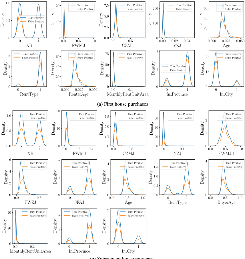
Figure 2: The distributions of each variable in the True Positive group (represented by the color blue) and the False Positive group (represented by the color orange), as predicted by ccGNN, are visualized for both datasets.
false positive group, which is shown in Figure 1 (c). This choice is motivated by the rationale outlined in Eq. (3), which indicates that real purchases are influenced by two factors: a common purchase factor and individual purchase factors. While the former can be modeled, the latter is inherently random and cannot be predicted. Figure 2 illustrates the distributions of each variable over the true positive group (blue curves) and false positive group (orange curves). Figure 2 (a) and (b) are the results of the first and subsequent purchase respectively. We then perform hypothesis testing on each variable.
To conduct the hypothesis testing on the house purchase, we utilize the results obtained from the best models. We evaluate variables within the true positive group and false positive group, as presented in Table 4 and Table 5.
Binomial Test The binomial test is employed in sampling statistics to evaluate whether the proportion of bivariate variables aligns with a specific hypothesis. The bivariate features encompass XB, RentType, SFAJ, In Province, and In City. It is noteworthy that all the features, with the exception of In Province (provincial native), hold significance in binomial tests, irrespective of whether it is the first or second phase of the prediction.
Mann Whitney U Test The Mann-Whitney U test is a widely employed non-parametric hypothesis test utilized to compare whether the medians of two independent samples are equivalent.
| Feature Name | Hypothesis Testing | P-value |
|---|---|---|
| XB | Binomial | 3.66e-23 |
| FWMJ | MannWhitney U | 9.03e-06 |
| CZMJ | MannWhitney U | 2.22e-17 |
| YZJ | F | 3.28e-08 |
| RentType | Binomial | 4.35e-229 |
| Age | Paired Sample- | 7.01e-300 |
| RenterAge | -MannWhitney U | 7.65e-248 |
| MonthlyRentUnitArea | F | 1.13e-15 |
| In Province | Binomial | 0.9054 |
| In City | Binomial | 1.75e-09 |
| Feature Name | Hypothesis Testing | P-value |
|---|---|---|
| XB | Binomial | 0.0689 |
| FWMJ | Paired Sample- | 0.0112 |
| FWMJ.1 | -MannWhitney U | 0.0211 |
| CZMJ | MannWhitney U | 0.0001 |
| FWZJ | MannWhitney U | 8.63e-19 |
| YZJ | F | 0.0006 |
| RentType | Binomial | 2.94e-06 |
| Age | Paired Sample- | 3.24e-188 |
| BuyerAge | -MannWhitney U | 7.73e-116 |
| SFAJ | Binomial | 0.0221 |
| MonthlyRentUnitArea | F | 0.0411 |
| In Province | Binomial | 0.8561 |
| In City | Binomial | 0.0007 |
Upon examining the distribution curves, the distributions of true positives and false positives exhibit substantial similarity across most continuum variables, except YZJ and MonthlyRentUnitArea. Consequently, the Mann-Whitney U test is conducted on all remaining continuum variables, yielding statistically significant results in each case.
In our analysis, we group two age-related variables together in a paired sample test to investigate the age gap or time interval between the rental period of the target group and the present time. Furthermore, with the inclusion of additional variables in the second prediction, we conduct an additional paired-sample test. This test aims to compare the size of the previously rented house with the size of the house purchased, thereby examining the housing level of residents before and after acquiring a property. The results show that all features are significant in both stages of housing purchase predictions.
FTest Since in terms of YZJ andMonthlyRentUnitArea, the distribution of true positives differs a lot from false positives, we decide to try variance-related tests. The distributions of both true and false positive samples of these two features basically obey normality, so we carry out the classic F test on them and the results turn out to be significant.
In the conducted hypothesis testing, we delved into the features of individuals who engage in their home purchases. Among those predicted to be first-time home purchasers, we note that all the features except for In Province are statically significant. This observation indicates that the decision to purchase a house for the first time is shaped by various common factors such as the gender of the buyer, the area of the rental house, the monthly rent, mortgage or not, and whether the individual is a native of the city, while an individual who is a native of the province or not seems to have not played a statistically significant role in this regard. Similarly, for those predicted subsequent house purchasers, the pattern repeats, with all features exhibiting statistical significance except for In Province.
The comprehensive hypothesis testing for all features across different housing buyers reveals the significant influence of common factors in driving home purchase decisions. It suggests that irrespective of first-time house purchases or subsequent house purchases, there are common and universal driving factors shaping these purchases. These common driving factors reflect broader social dynamics, economic landscapes, and cultural trends, collectively shaping the housing behavior of residents, and highlighting the interconnectedness between individuals, indicating that understanding these common driving factors is crucial for shaping future housing policies and the strategic planning of housing markets.
6 Conclusion
We believe that the driving forces behind residents' home purchases can be divided into two categories. The first category consists of universally existing driving forces, which are the common reasons that drive most people to buy a house. The second category encompasses individualized and random driving forces, making them difficult to predict. Therefore, modeling the first category of driving forces is advantageous for predicting housing transactions. By employing a factor model, we separate the common driving factors from all factors associated with housing purchases. Based on these factors, we construct a resident-to-resident relationship graph and propose a housing transaction prediction model using graph neural networks. In this model, the task of predicting whether a resident will make a home purchase is formulated as a graph node classification problem. We evaluate the model on two datasets: one representing transitions from renting to buying, and the other representing transitions from renting and buying to upgrading. The results indicate that the model achieves a sensitivity of over 80% in predicting housing transactions.
Acknowledgements
This work was supported by the Undergraduate Research and Learning Program of Southwestern University of Finance and Economics, No.YX220029.
@inproceedings{ijcai2024p810,
  title     = {Predicting Housing Transaction with Common Covariance GNNs},
  author    = {Li, Jinjin and Liu, Bin and Liu, Chengyan and Zhang, Hongli},
  booktitle = {Proceedings of the Thirty-Third International Joint Conference on
               Artificial Intelligence, {IJCAI-24}},
  publisher = {International Joint Conferences on Artificial Intelligence Organization},
  editor    = {Kate Larson},
  pages     = {7323--7330},
  year      = {2024},
  month     = {8},
  note      = {AI for Good},
  doi       = {10.24963/ijcai.2024/810},
  url       = {https://doi.org/10.24963/ijcai.2024/810},
}
TY - CPAPER TI - Predicting Housing Transaction with Common Covariance GNNs AU - Li, Jinjin AU - Liu, Bin AU - Liu, Chengyan AU - Zhang, Hongli T2 - Proceedings of the Thirty-Third International Joint Conference on Artificial Intelligence, IJCAI-24 PB - International Joint Conferences on Artificial Intelligence Organization PY - 2024 SP - 7323 EP - 7330 DO - 10.24963/ijcai.2024/810 UR - https://doi.org/10.24963/ijcai.2024/810 ER -Copied
Machine-readable versions of this paper, for tools and AI agents:





