
A Weighted-Based Fast Local Search for α-Neighbor p-Center Problem
Proceedings of the Thirty-Fourth International Joint Conference on Artificial Intelligence. Main Track. Pages 9005-9013.
https://doi.org/10.24963/ijcai.2025/1001
Keywords
- Search: S: Heuristic search
- Search: S: Combinatorial search and optimisation
- Search: S: Local search
Abstract
The α-neighbor p-center problem (α-pCP) is an extension of the classical p-center problem. It aims to select p centers from a set of candidate centers to minimize the maximum distance between any client and its α service centers. In this paper, we propose a weighting-based fast local search algorithm called WFLS for solving α-pCP. First, WFLS converts the complex α-pCP into a series of decision subproblems by specifying the service radius, effectively mitigating the gradient vanishing issue during the search process, and introduces a new MIP model. Then, it addresses the simpliffed subproblems using a fast local search procedure with a swap-based neighborhood structure. WFLS adopts an efffcient weighting strategy, an incremental evaluation technique, a reffned-grained penaltybased neighborhood evaluation, and two scoring functions of neighborhood evaluation to accelerate and guide the search process. Computational experiments on 154 widely used public benchmark instances demonstrate that WFLS outperforms the state-of-the-art methods in the literature. Speciffcally, WFLS improves 69 previous best known results and matches the best know results for all the remaining ones in less time than other competitors.
- [Albareda-Sambola et al., 2015] Maria Albareda-Sambola, Yolanda Hinojosa, Alfredo Marín, and Justo Puerto. When centers can fail: A close second opportunity. Computers and Operations Research, 62:145-156, 2015.
- [Calik and Tansel, 2013] Hatice Calik and Barbaros C Tansel. Double bound method for solving the p-center location problem. Computers and Operations Research, 40(12):2991-2999, 2013.
- [Cura, 2023] Tunchan Cura. A parallel mayfly algorithm for the α-neighbor p-center problem. Applied Soft Computing, 144:110527, 2023.
- [Drezner, 1987] Zvi Drezner. On the rectangular p-center problem. Naval Research Logistics, 34(2):229-234, 1987.
- [Elloumi et al., 2004] Sourour Elloumi, Martine Labbé, and Yves Pochet. A new formulation and resolution method for the p-center problem. INFORMS Journal on Comput- ing, 16(1):84-94, 2004.
- [Gaar and Sinnl, 2023] Elisabeth Gaar and Markus Sinnl. Exact solution approaches for the discrete α-neighbor p- center problem. Networks, 82(4):371-399, 2023.
- [Gao et al., 2015] Chao Gao, Xin Yao, Thomas Weise, and Jinlong Li. An efficient local search heuristic with row weighting for the unicost set covering problem. European Journal of Operational Research, 246(3):750-761, 2015.
- [Hakimi, 1964] S Louis Hakimi. Optimum locations of switching centers and the absolute centers and medians of a graph. Operational Research, 12(3):450-459, 1964.
- [Hochbaum and Shmoys, 1985] Dorit S Hochbaum and David B Shmoys. A best possible heuristic for the k- center problem. Mathematics of Operations Research, 10(2):180-184, 1985.
- [Ilhan et al., 2002] T Ilhan, F Ozsoy, and M Pinar. An effi- cient exact algorithm for the vertex p-center problem and computational experiments for different set covering sub- problems. Technical report, Bilkent University, Depart- ment of Industrial Engineering, 2002.
- [Irawan et al., 2016] Chandra Ade Irawan, Said Salhi, and Zvi Drezner. Hybrid meta-heuristics with vns and ex- act methods: application to large unconditional and con- ditional vertex p-centre problems. Journal of Heuristics, 22(4):507-537, 2016.
- [Kariv and Hakimi, 1979] Oded Kariv and S Louis Hakimi. An algorithmic approach to network location problems. I: The p-centers. SIAM Journal on Applied Mathematics, 37(3):513-538, 1979.
- [Khuller et al., 2000] Samir Khuller, Robert Pless, and Yoram J Sussmann. Fault tolerant k-center problems. The- oretical Computer Science, 242(1-2):237-245, 2000.
- [Krumke, 1995] Sven Oliver Krumke. On a generalization of the p-center problem. Information Processing Letters, 56(2):67-71, 1995.
- [Liu et al., 2020] Xiaolu Liu, Yuan Fang, Jiaming Chen, Zhouxing Su, Chumin Li, and Zhipeng Lü. Effective ap- proaches to solve p-center problem via set covering and sat. IEEE Access, 8:161232-161244, 2020.
- [López-Sánchez et al., 2019] Ana Dolores López-Sánchez, Jesús Sánchez-Oro, and Alfredo García Hernández-Díaz. GRASP and VNS for solving the p-next center problem. Computers and Operations Research, 104:295-303, 2019.
- [Martinich, 1988] Joseph S Martinich. A vertex-closing ap- proach to the p-center problem. Naval Research Logistics, 35(2):185-201, 1988.
- [Minieka, 1970] Edward Minieka. The m-center problem. SIAM Review, 12(1):138-139, 1970.
- [Mladenović et al., 2003] Nenad Mladenović, Martine Labbé, and Pierre Hansen. Solving the p-center problem with tabu search and variable neighborhood search. Networks, 42(1):48-64, 2003.
- [Pullan, 2008] Wayne Pullan. A memetic genetic algorithm for the vertex p-center problem. Evolutionary Computa- tion, 16(3):417-436, 2008.
- [Reinelt, 1991] Gerhard Reinelt. Tsplib-a traveling sales- man problem library. ORSA Journal on Computing, 3(4):376-384, 1991.
- [Sánchez-Oro et al., 2022a] Jesús Sánchez-Oro, A. D. López-Sánchez, Alfredo García Hernández-Díaz, and Abraham Duarte. Grasp with strategic oscillation for the α-neighbor p-center problem. European Journal of Operational Research, 303(1):143-158, 2022.
- [Sánchez-Oro et al., 2022b] Jesús Sánchez-Oro, AD López- Sánchez, Alfredo García Hernández-Díaz, and Abraham Duarte. Grasp with strategic oscillation for the α-neighbor p-center problem. European Journal of Operational Re- search, 303(1):143-158, 2022.
- [Su et al., 2021] Zhouxing Su, Qingyun Zhang, Zhipeng Lü, Chu-Min Li, Weibo Lin, and Fuda Ma. Weighting-based variable neighborhood search for optimal camera place- ment. In Thirty-Fifth AAAI Conference on Artificial Intel- ligence, AAAI 2021, pages 12400-12408, 2021.
- [Toregas et al., 1971] Constantine Toregas, Ralph Swain, Charles ReVelle, and Lawrence Bergman. The location of emergency service facilities. Operational Research, 19(6):1363-1373, 1971.
- [Yin et al., 2017] Ai-Hua Yin, Tao-Qing Zhou, Jun-Wen Ding, Qing-Jie Zhao, and Zhi-Peng Lv. Greedy random- ized adaptive search procedure with path-relinking for the vertex p-center problem. Journal of Computer Science and Technology, 32(6):1319-1334, 2017.
- [Zhang et al., 2020] Qingyun Zhang, Zhipeng Lü, Zhoux- ing Su, Chumin Li, Yuan Fang, and Fuda Ma. Vertex weighting-based tabu search for p-center problem. In Pro- ceedings of the Twenty-Ninth International Joint Confer- ence on Artificial Intelligence, IJCAI 2020, pages 1481- 1487, 2020. IJCAI
- [Zhang et al., 2022] Qingyun Zhang, Zhouxing Su, Zhipeng Lü, and Lingxiao Yang. A weighting-based tabu search algorithm for the p-next center problem. In Proceedings of the Thirty-First International Joint Conference on Arti- ficial Intelligence, IJCAI 2022, pages 4828-4834, 2022. IJCAI
References were extracted automatically from the PDF and may contain errors.
Full text extracted automatically from the PDF; figures, tables and equations may differ. The PDF is the version of record.
1 Introduction
The p-center problem is a well-known problem in the field of combinatorial optimization, which has been proven to be NP-hard [Kariv and Hakimi, 1979]. It involves finding p centers in a given set of candidate centers, such that the maximum distance from any demand client to its nearest center is minimized. The p-center problem has a wide range of applications, such as the problems of determining the locations of emergency centers [Toregas et al., 1971], hospitals [Hakimi, 1964], and fire stations [Drezner, 1987] to serve the communities. In the last 50 years, the p-center problem has been wide studied in academic society. There are mainly three kinds of methodologies, including exact algorithms [Minieka, 1970; Ilhan et al., 2002; Elloumi et al., 2004; Calik and Tansel, 2013; Liu et al., 2020], approximation algorithms [Hochbaum and Shmoys, 1985; Martinich, 1988], and metaheuristic algorithms [Mladenovi´c et al., 2003; Pullan, 2008; Irawan et al., 2016; Yin et al., 2017; Zhang et al., 2020].
∗Corresponding Author
However, a center may be forced to close due to an unpredictable incident, such as natural disasters, sudden system failures. In this case, the clients served by the reference center have to turn to other backup centers as quickly as possible. This issue has been classified into two cases based on whether the client can obtain information about center faults in advance. In the first case, the client cannot know the fault information and must first arrive at the closest center and then to the next one. This scenario is described as the p-next center problem [Albareda-Sambola et al., 2015; Zhang et al., 2022]. In the second case, the client can know the fault information in advance. At this time, the client can directly move to the nearest available backup center, which is the α-neighbor p-center problem (α-pCP) that this paper focuses on studying. With the increasing convenience of information sharing, the importance of the α-pCP is growing.
Krumke [1995] first introduced the α-pCP, which occurs in many industrial applications and has been proven to be NPhard [Kariv and Hakimi, 1979]. Its aim is to locate p centers from a set of candidate centers and assign up to α centers to each client, such that the maximum distance of each client to its assigned centers is minimized. The closest center serves as the primary reference center, while the second to the αth nearest centers act as backup centers. For the α-pCP, the given vertices not only are the clients but also the candidate centers. Figure 1 shows an illustrative diagram of the α-pCP, where Figure 1(a) is the original graph and Figure 1(b) is a solution of p = 3, α = 2.
In previous years, the study of the α-pCP focused on the theoretical study of approximation algorithms. Krumke [1995] introduced different formulations for α-pCP
4. Khuller et al. [2000] presented two approximation algorithms. The first achieves an approximation factor of 3 for any α, and the second with an approximation factor of 2 for α < 4. Based on [Krumke, 1995] and [Khuller et al., 2000], L´opez-S´anchez et al. [2019] proposed a 2-approximation algorithm to further improve the quality of the solution.
In addition to theoretical studies, some practical studies of exact and heuristic algorithms have been introduced in recent years. S´anchez-Oro et al. [2022a] introduced a metaheuristic algorithm, which combines a greedy randomized adaptive search procedure with tabu search, and a strategic oscillation (SO) post-processing procedure to ensure high solution quality to the α-pCP. Cura [2023] proposed a competitive algorithm that combines the mayfly optimization algorithm (MA) with a local search procedure for the α-pCP. Gaar and Sinn [2023] presented two integer programming formulations and developed a branch-and-cut algorithms for the α-pCP. To the best of our knowledge, it is the most recent and best performing method currently to solve the α-pCP.
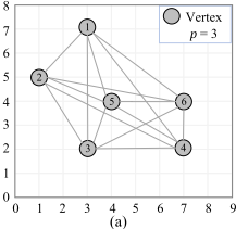
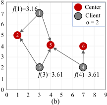
In this paper, we present a weighting-based fast local search (WFLS) algorithm to solve the α-pCP. Unlike previous metaheuristics that directly optimize the original problem, WFLS transforms the original α-pCP into a series of decision subproblems by specifying a serving radius. These subproblems are then efficiently solved using a weighting-based fast local search procedure that adopts a swap-based neighborhood structure and an incremental neighborhood evaluation technique based on a refined-grained penalty strategy.
The main contributions of our work are as follows:
- We propose a novel approach that transforms the αneighbor p-center optimization problem into a series of decision subproblems, introducing a new decisionbased MIP model. We obtain the solution to the original problem by sequentially solving these subproblems. It smooths the solution space and prevents gradient vanishing, enhancing the effectiveness of local search-based algorithms to solve the α-pCP.
- We introduce a weighting technique for local search, resulting in an effective search procedure called weighting-based fast local search (WFLS), which increases search diversity and allows the algorithm to escape from the local optimal trap.
- WFLS algorithm employs a new neighborhood structure based on a dedicated swap move comprising a closing operation and an opening operation. In addition, we use a new refined-grained penalty strategy for neighborhood evaluation, two scoring functions to guide the neighboring search, and an incremental evaluation strategy to improve the efficiency of the search.
- Tested on 154 classical instances of the α-pCP, WFLS algorithm improves the best known results for 69 instances and matches on all the remaining ones in the
literature, respectively. In addition, the computational time of WFLS is much shorter than that of the state-ofthe-art algorithms in the literature.
2 ProblemDescription and Transformation
Given an undirected complete graph G = (V, E), where V = {1, 2, ..., n} is the vertex set and E = {(i, j)|i, j ∈ V } is the edge set. dij denotes the distance between each pair of vertices i and j. The α-pCP aims to select a center subset C (|C| = p) from the set V to minimize the maximum distance between each client i ∈ (V \ C) and its α serving centers.
Based on the above notations, the classical mixed-integer programming (MIP) model [Gaar and Sinnl, 2023] for the αpCP can be formulated as follows.
x and y are decision variables, where xj = 1 iff a candidate center j ∈ V is opened, yij = 1 iff client i ∈ V is served by candidate center j, and r ∈ R+ denotes the upper bound of the serving radius. Objective (1) is intended to minimize the service radius. Constraint (2) restricts the number of opened centers to be no more than p. Constraints (3) ensure that each vertex is either assigned to exactly α centers or opened to be a center. Constraints (4) restrict that only those centers that are in an open state can serve the client vertices. Constraints (5) ensure that the radius r is not less than the length of any arc from each client to its all α serving centers.
Obviously, to obtain the optimal serving radius, there is at least one equality in Constraints (5), i.e., the optimal serving radius of a specific α-neighbor p-center instance must be the same as the length of a certain edge dij . Let R = {dij |i, j ∈ V } = {r1, r2, . . . , rm} be the ordered list containing all distinct values of dij , where r1 < r2 < ... < rm. The α-pCP is to find the rank q of the smallest radius on R such that the model is still feasible after adding a constraint r ≤ rq, but it becomes infeasible if we add constraint r ≤ rq-1.
Problem Transformation. Based on the above analysis, the α-pCP can be solved by finding feasible solutions to a series of subproblems with the given radius. Specifically, it is transformed into decision subproblems where serving arcs are bounded by r, and centers need to be located under the constraint that the actual radius does not exceed r. Therefore, the focus is limited to center-client pairs with distances not exceeding the current radius r. In detail, we employ a vertex set Sq j = {i ∈ V |dij ≤ rq, i ̸= j} to represent the set of clients that candidate center j ∈ V can serve within covering radius rq, or the set of candidate centers that can serve the
Algorithm 1 The main framework of the WFLS algorithm
Input A graph G, the center number p, the value of α Output The best solution found so far X∗
- 1: iter ← 1, vertex weights wi ← 1, ∀i ∈ V
- 2: The age aj ← 0, ∀j ∈ V
- 3: Current solution X, initial radius rq ← Initialize(G, p)
- 4: Previous solution X′ ←X, X∗ ←X
- 5: The radius order list R = {r1, r2, ..., rq}
- 6: while Termination condition is not met do
- 7: q ← q -1, update the set of illegal vertices I(X)
- 8: while The time limit is not reached and |I(X)| > 0 do
- 9: (i, j) ← find the best swap move /* Algorithm 2 */
- 10: X ←X ∪ {i} \ {j}
- 11: if |I(X)| = 0 then
- 12: X∗ ← X
13:
else if (|I(X)| > |I(X′ )| then
- 15: end if
- 16: X′ ←X, iter ← iter +1
- 17: end while
- 18: end while
- 19: return X∗
client j. Therefore, with the optimal edge length rank q specified, the new reformulated model (α-pCPq) can be defined by Eqs. (8)-(11), where ui is a binary variable that equals 1 if client i is not covered by at least α centers, and xj is the same decision variable as in the model (α-pCP).
Model (α-pCPq) minimizes the number of uncovered vertices by exactly opening p centers as shown in objective function (8). Constraints (9) ensure that for each vertex, there are at least α centers within the covering radius rq or it is opened to be a center. We need to traverse the distinct edge length list R to examine each possible covering radius.
3 VertexWeighting-Based Local Search
3.1 General Framework
To address the α-pCP, we transform it into a series of decision subproblems for a given radius and solve these subproblems using the weighting-based fast local search (WFLS). Firstly, it adopts a greedy constructive heuristic algorithm to obtain an initial feasible solution and the upper bound of the radius. Subsequently, WFLS converts α-pCP into a series of rq-radius α-pCP decision subproblems and solves them by a fast local search procedure combining with a weighting technique. As soon as the rq-radius α-pCP is solved, we decrease rq by setting rq to rq-1 and solve the resulting subproblem once again. In practical applications, these subproblems can actually be solved in parallel.
Specifically, Algorithm 1 outlines the main framework of WFLS. It starts by generating an initial solution X with an initial radius rq using a greedy construction algorithm under the principle of minimizing the objective (1) (line 3). Using the initial radius rq, we initialize the ordered radius list R with all distance lengths (line 5). Then, the model (α-pCPq) is solved by decreasing q to q - 1 in turn until it fails to find any feasible solution for model (α-pCPq-1) within the given time limit. For each subproblem, we record the set of client vertices that are not fully covered by α centers, and define it as the illegal vertices set I(X). This set is iteratively optimized by fast local search until |I(X)| = 0 or the time limit is reached (lines 8-17).
3.2 Reduction Rule
To simplify the original graph and reduce the scale of the search space, we develop a reduction rule to simplify the graph. Specifically, we fix some centers that must be included in the optimal solution. Since each vertex can be both a client and a center, if there exists vertex k whose number of candidate centers that can cover it within the given radius is less than α, i.e., |Sk| < α, then vertex k must be a center in order to find a feasible solution.
3.3 Reformulation andWeighting Technique
The weighting technique helps the search to escape from local optimum by introducing an adaptive objective function. The weighting strategy has been successfully applied to many problems, such as the single-cost set cover problem [Gao et al., 2015], the classical p-center problem [Zhang et al., 2020], and the optimal camera placement problem [Su et al., 2021]. We transform the α-pCP into a series of decision subproblems to determine whether all client vertices can be assigned to α centers within a specific r-radius. To effectively solve each subproblem, the constraint requiring each vertex to be assigned to α centers within the radius r or opened to be a center is relaxed, and a penalty is imposed for each illegal vertex in the objective function.
Specifically, let wi be the weight of vertex i, the objective function f(X) can be defined as Eq. (12), which is the sum of the weights of each illegal vertex.
The initial weight assigned to each vertex is set to 1. During subsequent searches, if WFLS fails to reduce the number of illegal vertices, it indicates that the search is trapped in a local optimum. To address this issue, WFLS increases the weight wk of each illegal vertex k ∈ I(X) ⊂ V by one unit when the search falls into local optimum (Algorithm 1, lines 13-15).
In the later stage of the search, once stagnation is encountered, the weight of the corresponding illegal vertices is increased, and the more times a vertex appears in I(X), the greater its weight will be. The weighting strategy changes
Algorithm 2 Find the best swap move
Input Current solution X, the set of illegal vertices I(X), the number of iteration iter, the age a of candidate centers Output The best swap move (i∗ , j ∗ )
- 1: Best swap move (i∗ , j ∗ ) ←∅, ∆f ∗ 1 ←+∞
- 2: k ←a random vertex in I(X)
- 3: for all i ∈ Sk \X ∪ {k} do
- 4: Virtually update Scorej, {j ∈ Sv ∩ X|v ∈ Si, cv = α + 1}, which affects the calculation of ∆f1(i, j)
- 5: for all j ∈ X do
- 6: j is not the recently-opened center
- 7: if (∆f1(i, j) < ∆f ∗ 1 ) or ((∆f1(i, j) = ∆f ∗ 1 ) ∩ (ai > a∗i )) then
- 8: ∆f ∗ 1 ← ∆f1(i, j), (i∗ , j ∗ ) ← (i, j)
- 9: end if
- 10: end for
- 11: end for
- 12: Return (i∗ , j ∗ )
the landscape of the solution space, thus effectively preventing vertices from remaining illegal for following periods.
3.4 Neighborhood Structure and Evaluation
The neighborhood structure defines the set of solutions adjacent to a given solution in the solution space. For the current solution X, a neighborhood move move generates a new solution X ⊕ move. To tackle each rq-radius α-pCP subproblem, WFLS adopts a swap-based neighborhood structure. Specifically, a swap move consists of opening a center i ∈ V \ X and closing a center j ∈ X, denoted as move(i, j). At each iteration, based on the incumbent solution X, WFLS tries to improve X by selecting the bestimprovement move to produce a new neighborhood solution X ⊕ move(i, j) = X ∪ {i} \ {j}.
The neighborhood evaluation is an essential and the most time-consuming part of trajectory-based metaheuristic algorithms. To improve the incumbent solution X and optimize the objective value, the local search procedure follows a bestimprovement policy, evaluating all neighborhood moves and selecting the one that leads to the best neighboring solution. Evaluating a neighborhood move involves calculating the weighted sum of illegal vertices, as specified by Eq. (12). If the weighted sum is naively calculated, the time complexity is O(p · (n - p)). Since there are totally O(p · (n - p)) neighborhood moves, the neighborhood evaluation complexity of a round of local search is O((p · (n - p))2 ), making the process quite time-consuming, especially for large scale instances. To enhance efficiency without sacrificing the solution quality, WFLS adopts three acceleration and guiding strategies, which include a refined-grained penalty strategy for neighborhood evaluation, an incremental evaluation technique, and two scoring functions.
Refined-grained penalty strategy. WFLS uses a refinedgrained penalty strategy to reformulate the neighborhood evaluation function, providing a more nuanced evaluation approach. Instead of classifying the client status directly as legal or illegal, we assign penalties to illegal clients based on the number of centers currently covering them. The more centers there are that can cover a client, the easier it is to be fully covered by α centers, and thus the smaller the penalty factor will be. Conversely, fewer covering centers result in a larger penalty factor. To capture this distinction, we use varying penalty factors for illegal vertices. Specifically, the distance to legal covering is used as the penalty factor, i.e., α - ck. The new neighborhood evaluation function is presented in Eq. (13),
where ck denotes the number of centers currently covering client k, i.e., ck = |Sk ∩X|. This penalty strategy provides a finer-grained neighborhood evaluation and prioritizes the full covering of more difficult illegal clients, leading to improved solutions by directing the search more efficiently.
Incremental evaluation technique. To accelerate the neighborhood evaluation procedure, WFLS adopts an incremental evaluation mechanism to efficiently evaluate neighborhood moves instead of naively calculating the reformulated objective by Eq. (13). Specifically, since there are only small changes from the current solution to a neighboring solution, the objective of a neighboring solution can be calculated incrementally by the variation of closing a center i and opening a center j, i.e., f(X ⊕move(i, j)) = f(X) +∆f(i, j), where ∆f represents the increment of the objective value after performing a swap move. WFLS uses Score to record the (potential) contribution of each (candidate) center to the current solution, enabling rapid incremental evaluation of the objective value based on Score. Score is defined and calculated according to Eq. (14).
For an opening center j ∈ X, Scorej is the sum of the weights of clients that j can cover, which is either not fully covered or exactly covered by α centers, i.e., ck ≤ α; For a closing center j /∈ X, Scorej is the sum of the weights of nofully covered clients that j can cover. When ck > α, center j does not contribute to the current client k that can be covered, as closing it leaves k still legally covered. It is worth noting that since the vertices are both convertible between the center and the client, the calculation of the contribution values needs to take themselves into account. To facilitate the calculation of Score, we categorize the clients into three states, ck < α, ck = α, and ck > α. According to the definition of Score, its value needs to be updated only when the state of the client changes. Obviously, opening a center i causes clients with ck = α - 1 to transfer to ck = α, and clients with ck = α to transfer to ck > α. Conversely, closing a center j causes clients with ck = α + 1 to transfer to ck = α, and clients with ck = α to transfer to ck < α. Thus, when trying to open i and close j, the increment of the neighborhood move is calculated as Eq. (15).
| Instances with α = 2 (77) | Instances with α = 3 (77) | |||||||||
|---|---|---|---|---|---|---|---|---|---|---|
| Alg. | #best | #B/#E/#W | Gap (%) | p-value | CPU (s) | #best | #B/#E/#W | Gap (%) | p-value | CPU (s) |
| SO (2022) | 5 | 72/5/0 | 9.68 | 1.79E-13 | 841.46 | 2 | 75/2/0 | 8.56 | 5.74E-14 | 975.58 |
| MA (2023) | 13 | 64/13/0 | 7.56 | 3.75E-12 | 821.06 | 13 | 64/13/0 | 5.85 | 3.75E-12 | 938.86 |
| 1HSVL (2023) | 28 | 49/28/0 | 19.46 | 1.15E-09 | 1178.08 | 25 | 52/25/0 | 20.80 | 3.65E-10 | 1329.72 |
| 2HVSL (2023) | 42 | 35/42/0 | 3.08 | 2.52E-07 | 872.89 | 46 | 36/41/0 | 4.20 | 1.71E-07 | 1083.39 |
| Gurobi (α-pCPq) | 63 | 14/63/0 | 0.10 | 1.48E-03 | 664.18 | 54 | 23/54/0 | 0.16 | 2.72E-05 | 690.19 |
| WFLS | 77 | - | 0 | - | 16.98 | 77 | - | 0 | - | 20.11 |
Two scoring functions. During neighborhood evaluation, using only the objective function often results in multiple best neighboring solutions. To address this issue, WFLS employs two scoring functions. The primary scoring function minimizes the refined-grained weighted sum of illegal vertices, as this aligns with the redefined optimization objective as defined in Eq. (13). To further distinguish multiple best swap moves with the same primary score and effectively mitigate the gradient vanishing issue, WFLS uses a secondary scoring function. The age ai of center i refers to the number of iterations since it has been last closed. For two solutions having the same weighted sum of illegal vertices, preferring the opening of older candidate centers helps the search to explore new configurations and enhances the search diversification, which is usually more promising to improve the current solution. Therefore, WFLS introduces the age as the secondary scoring function. Specifically, for a move move(i, j) producing a neighboring solution X, it is calculated as follows:
where i∗ denotes the open center of the best swap move (i∗ , j ∗ ). At each iteration, WFLS selects the best swap move with the smallest ∆f1 value, and breaks ties by choosing the move with the largest ∆f2 value.
In addition, to prevent immediately re-closing the recentlyopened center, the recently-opened center will not be evaluated and selected at the next iteration.
Algorithm 2 presents the neighborhood evaluation procedure for the α-pCP, where each vertex can be legalized as either a client (requiring α assigned centers) or as a center. Our WFLS considers both these two cases in the neighborhood evaluation (line 3).
3.5 Neighborhood Reduction
To accelerate the neighborhood search, WFLS proposes one neighborhood reduction strategy.
WFLS restricts to choose the candidate centers by focusing on a single illegal client at a time. As we know, the objective value can only be improved by covering the vertices in I(X) or opening them as centers, so WFLS evaluates a swap move move(i, j) only if i ∈ I(X) or can cover some vertices in I(X). For the rq-radius α-pCP subproblem, since each client must be eventually fully covered by at least α centers, WFLS randomly selects a vertex k ∈ I(X), and evaluates only neighborhood moves move(i, j) where i ∈ Sk and j ∈ X. The approach significantly reduces the neighborhood size from O(p · (n-p)) to O(p · |Sk|), with the side effect of enhancing the search diversification.
4 Experiments and Analysis
To evaluate the performance of WFLS, we conduct extensive experiments on 154 public benchmark instances and compare WFLS with the state-of-the-art algorithms in the literature, such as SO [S´anchez-Oro et al., 2022b], MA [Cura, 2023], and 1HSVL and 2HVSL [Gaar and Sinnl, 2023].
4.1 Experimental Benchmarks and Protocol
There are 154 instances with α = 2, 3 for the α-pCP generated from TSP-Library [Reinelt, 1991]. The vertex number n varies from 48 to 1323, and the center number p ranges from 10 to 140. In these instances, location is given in twodimensional coordinates, and distances between any two vertices i, j are calculated using the Euclidean metric.
Our WFLS is coded in C++ and all our experiments are carried out on Windows Server 2019 x64 with an Intel Xeon Gold 6133 2.50GHz CPU. For each instance, we carried out 20 independent runs under 180 seconds time limit. The computational platform for the reference algorithms 1HSVL and 2HVSL is an Intel Xeon E5-2670v2 machine with 2.5GHz and 6GB of RAM, and the time limit for each instance is 1800 seconds. The reference algorithms MA and SO are tested on an Apple M2 Pro 12-core 3480 MHz computer with 16GB RAM running MacOS Ventura and the time limit is 1800 seconds. Compared to the reference algorithms, the maximum runtime of our algorithm is reduced by a factor of 10. Moreover, our algorithm has converged within this time limit, and extending the running time has almost no impact on the results. It shows the high efficiency of our algorithm. Notably, there are no parameters that need to be tuned in our WFLS.
4.2 Computational Results
To test the performance of WFLS, we report the detailed performance metrics and results in Tables 1 and 2.
"Instances with α = 2 (77)" and "Instances with α = 3 (77)" represent the group of instances whose neighbor α = 2 and α = 3, respectively, with a total of 77 instances in each group. Column Instance gives the instance names. Columns n and p report the numbers of vertices and centers, respectively. Column Gap indicates the average gap between the results obtained by the corresponding algorithm and the best results on the current set of instances. Column CPU shows the average CPU execution time in seconds. For our WFLS, the CPU time includes the total time for computing the initial solution and solving all the decisions. Column UB represents the best upper bound obtained by these algorithms, and the numbers in bold stand for the best known results. Column #best shows the number of instances where the corresponding algorithms match the best known results. Columns #B, #E, and #W indicate the number of instances where our WFLS obtains better, equal, and worse results compared to the corresponding algorithms, respectively. To verify the statistical significance of the comparison between WFLS and the reference algorithms, we give the p-values by the non-parametric Wilcoxon test in column p-value, where a p-value less than
| Instance | n | α = 2 | α = 3 | |||||||||||
|---|---|---|---|---|---|---|---|---|---|---|---|---|---|---|
| p | MA | 1HSVL/2HVSL | WFLS | MA | 1HSVL/2HVSL | WFLS | ||||||||
| UB | CPU (s) | UB | CPU (s) | UB | CPU (s) | UB | CPU (s) | UB | CPU (s) | UB | CPU (s) | |||
| pr439 | 439 | 70 | 806.23 | 650.64 | 726.72 | 1050.05 | 726.72* | 0.75 | 1027.74 | 837.88 | 1006.23 | TL | 1005.61 | 0.86 |
| pr439 | 439 | 80 | 781.55 | 784.97 | 637.38 | TL | 637.38* | 0.86 | 975 | 881.52 | 915.49 | TL | 905.88 | 1.29 |
| pr439 | 439 | 90 | 721.11 | 826.21 | 583.1 | 24.75 | 583.1* | 0.57 | 901.39 | 958.18 | 813.94 | TL | 797.26 | 1.04 |
| rat575 | 575 | 10 | 116.1 | 151.27 | 116.1 | 24.75 | 116.1* | 0.85 | 138.85 | 437.17 | 138.85 | 19.41 | 138.85* | 1.59 |
| rat575 | 575 | 20 | 73 | 290.76 | 72.62 | 265.55 | 72.4* | 2.14 | 94.41 | 840.29 | 93.43 | 705.69 | 93.43* | 2.20 |
| rat575 | 575 | 30 | 59.91 | 806.14 | 59.14 | TL | 57.57 | 8.22 | 73.24 | TL | 72.09 | TL | 72.01 | 4.04 |
| rat575 | 575 | 40 | 51 | 1061.96 | 50.25 | TL | 48.75 | 8.49 | 64.07 | TL | 66.61 | TL | 61.98 | 15.12 |
| rat575 | 575 | 50 | 46.52 | 1350.20 | 45.88 | TL | 42.72 | 12.23 | 57.45 | TL | 57.25 | TL | 53.46 | 19.21 |
| rat575 | 575 | 60 | 41.59 | 1535.83 | 41.15 | TL | 38.47 | 22.49 | 51.92 | TL | 53.74 | TL | 48.27 | 26.19 |
| rat575 | 575 | 70 | 39.12 | 1733.20 | 37.48 | TL | 35.47 | 12.89 | 49.04 | TL | 47.42 | TL | 44.38 | 5.74 |
| rat575 | 575 | 80 | 35.9 | TL | 34.99 | TL | 32.76 | 76.25 | 45.28 | TL | 45.28 | TL | 40.72 | 29.70 |
| rat575 | 575 | 90 | 35.06 | TL | 32.45 | TL | 30.41 | 73.42 | 42.95 | TL | 44.69 | TL | 38.01 | 20.14 |
| rat575 | 575 | 100 | 33.6 | TL | 30 | TL | 28.79 | 39.83 | 39.96 | TL | 40.79 | TL | 35.85 | 56.37 |
| rat783 | 783 | 10 | 136.01 | 251.14 | 135.25 | 34.92 | 135.25* | 1.22 | 163.68 | 511.48 | 163.68 | 54.58 | 163.68* | 0.19 |
| rat783 | 783 | 20 | 84.08 | 427.90 | 83.1 | 25.68 | 83.1* | 1.79 | 110.54 | 983.14 | 109.57 | 841.93 | 109.57* | 5.40 |
| rat783 | 783 | 30 | 69.64 | 1178.00 | 67.88 | TL | 67.12* | 2.43 | 87.09 | TL | 83.55 | TL | 83.55* | 4.59 |
| rat783 | 783 | 40 | 59.36 | 1600.20 | 57.43 | TL | 55.95* | 24.73 | 74.71 | TL | 76.9 | TL | 71.85 | 31.71 |
| rat783 | 783 | 50 | 54.23 | TL | 55.04 | TL | 50.54 | 28.50 | 67.23 | TL | 68.66 | TL | 62.68 | 30.04 |
| rat783 | 783 | 60 | 51.35 | TL | 49.04 | TL | 45.22 | 57.42 | 60.67 | TL | 61.4 | TL | 55.97 | 90.83 |
| rat783 | 783 | 70 | 45.8 | TL | 44.2 | TL | 41.34 | 106.36 | 57.08 | TL | 59.03 | TL | 51.92 | 24.78 |
| rat783 | 783 | 80 | 43.14 | TL | 41.68 | TL | 38.29 | 26.90 | 54.04 | TL | 56.14 | TL | 48.37 | 117.71 |
| rat783 | 783 | 90 | 41.01 | TL | 40.36 | TL | 36.06 | 17.41 | 49.58 | TL | 50.49 | TL | 44.94 | 71.11 |
| rat783 | 783 | 100 | 39.12 | TL | 37.64 | TL | 33.97 | 43.00 | 47.51 | TL | 47.76 | TL | 42.2 | 87.14 |
| pr1002 | 1002 | 10 | 3853.89 | 684.83 | 3853.89 | 48.07 | 3853.89* | 0.73 | 5254.05 | 1547.96 | 5202.16 | 107.49 | 5202.16* | 17.82 |
| pr1002 | 1002 | 20 | 2630.59 | 970.62 | 2593.26 | TL | 2583.12* | 5.05 | 3203.9 | 1283.98 | 3170.57 | 135.59 | 3170.57* | 1.91 |
| pr1002 | 1002 | 30 | 2110.09 | 1219.19 | 2059.73 | TL | 2040.22 | 27.01 | 2651.89 | 1650.35 | 2631.54 | TL | 2580.7 | 13.52 |
| pr1002 | 1002 | 40 | 1839.84 | 1491.82 | 1746.42 | TL | 1711.72 | 26.73 | 2304.89 | TL | 2210.2 | TL | 2170.83 | 12.10 |
| pr1002 | 1002 | 50 | 1662.08 | 1721.68 | 1523.15 | TL | 1503.8 | 10.31 | 2018.04 | TL | 2015.56 | TL | 1882.82 | 8.57 |
| pr1002 | 1002 | 60 | 1498.33 | TL | 1403.57 | TL | 1346.29 | 17.37 | 1892.75 | TL | 1874.17 | TL | 1729.29 | 56.05 |
| pr1002 | 1002 | 70 | 1389.24 | TL | 1372.95 | TL | 1237.94 | 45.27 | 1750 | TL | 1732.77 | TL | 1565.25 | 65.55 |
| pr1002 | 1002 | 80 | 1346.29 | TL TL | 1253.99 | TL | 1131.37 | 23.75 | 1656.05 | TL | 1565.25 | TL | 1424.59 | 65.20 |
| pr1002 | 1002 | 90 | 1264.91 | 1131.37 | TL | 1053 | 17.85 | 1517.93 | TL | 1431.36 | TL | 1334.17 | 54.19 | |
| pr1002 | 1002 | 100 | 1202.08 | TL | 1070.05 | TL | 999.64 | 43.22 | 1450.86 | TL | 1414.21 | TL | 1251 | 63.12 |
| rl1323 | 1323 | 10 | 4554.09 | 691.75 | 4554.09 | 660.59 | 4554.09* | 2.39 | 6229.6 | 765.02 | 6229.6 | TL | 6229.6* | 3.37 |
| rl1323 | 1323 | 20 | 3079.56 | 979.50 | 3055.56 | TL | 3036* | 7.70 | 3852.82 | 1415.16 | 3845.66 | TL | 3845.66* | 5.44 |
| rl1323 | 1323 | 30 | 2520.7 | 1361.84 | 2913.42 | TL | 2399.02* | 20.70 | 3102 | 1777.78 | 3906.16 | TL | 3036.61 | 46.69 |
| rl1323 | 1323 | 40 | 2090.87 | TL | 2039.56 | TL | 2011.46 | 27.12 | 2661.54 | TL | 2562.35 | 80.34 | ||
| rl1323 | 1323 | 50 | 1927.09 | TL | 1958.61 | TL | 1762.56 | 47.96 | 2430.27 | TL | 2652.14 | TL | 2226.88 | 76.73 |
| rl1323 | 1323 | 60 | 1760 | TL | 1710.6 | TL | 1597.72 | 136.55 | 2115.13 | TL TL | 2308.32 2495.02 | TL | 2000.23 | 40.09 |
| 1323 | 70 | 1587.15 | TL | 1647.07 | 1449.41 | 73.71 | 2021.87 | 1973.72 | TL TL | 1812.9 | 97.90 | |||
| rl1323 rl1323 | 1323 | 80 | 1511.32 | TL | 1536 | TL | 1328 | 55.87 | 1870.03 | TL TL | 1918.35 | TL | 1699.89 1587.15 | 71.72 49.95 |
| rl1323 rl1323 | 1323 | 90 | 1423.38 | TL | 1329.66 | TL TL | 1235.74 | 100.85 | 1745.58 | TL TL | 1751.21 | |||
| Gap | 1323 | 100 | 1330.32 | TL | 1278.1 | TL | 1159.54 | 41.56 | 1655.13 | 1624.22 | TL | 1475.21 | 44.32 | |
| 9.53% | 5.52% | 7.52% | ||||||||||||
| 0 | 7.2% | 0 | ||||||||||||
0.05 indicates a significant difference In addition, based on model (α-pCPq), we find the optimal objective value for some instances using the Gurobi 11.0.3 solver with 1800 seconds time limit per instance, which matches the time limit used in the 1HSVL/2HVSL exact algorithm. The proven optimal objective values are marked with '*'.
Table 1 summarizes the overall results on all the instances obtained by SO, MA, 1HSVL, 2HVSL, and our WFLS and Gurobi (α-pCPq). It is evident that WFLS achieves the best known results on all the 154 instances (Gap = 0). Specifically, compared to the best-performing algorithm 2HVSL, WFLS obtains 35 better, 42 equal, and no worse solutions for

| Instances with α = 2 (40) | Instances with α = 3 (40) | |||||
|---|---|---|---|---|---|---|
| Alg. | #B/#E/#W | UB | CPU (s) | #B/#E/#W | UB | CPU (s) |
| WFLSNW | 28/12/0 | 1066.01 | 155.01 | 32/8/0 | 1364.59 | 159.93 |
| WFLSf2 | 14/26/0 | 998.68 | 52.65 | 21/18/1 | 1286.51 | 48.26 |
| WFLSw | 30/10/0 | 1097.96 | 131.33 | 35/5/0 | 1414.36 | 136.64 |
| WFLSRP | 34/6/0 | 992.31 | 57.14 | 30/10/0 | 1278.31 | 74.35 |
| WFLS | - | 977.12 | 32.44 | - | 1253.74 | 38.28 |
"α = 2" group, and 31 better, 46 equal and no worse solutions for "α = 3" group. The maximum p-value is much less than 0.05, further indicating the superiority of WFLS in terms of the quality of solution. Moreover, WFLS has the shortest average CPU time, with 16.98 (20.11) seconds for α = 2 (3), while the average CPU times of all the reference algorithms exceed 500 seconds. It shows that WFLS outperforms all reference algorithms in terms of both solution quality and computational efficiency across all instances.
Table 2 summarizes detailed experimental results for improved instances and large-scale challenging instances with more than 500 vertices, comparing our algorithm with the top performers (MA, 1HSVL, and 2HVSL) 1 . From Table 2, we can observe that the proposed WFLS improves the previous best known results and outperforms all reference algorithms on these large instances in terms of computing time. For the remaining 68 instances, WFLS matches the optimal or the best known solutions. On large instances, the average gap between the best results obtained by WFLS and the best results found by all the algorithms (including ours) is 0, while for other competitors, the average gap is larger than 5%. It is important to note that even a 1% gap is considered to be significant due to the large value of UB for large graphs. Furthermore, compared to the best 1HSVL and 2HVSL exact algorithms, our model (α-pCPq) can prove the optimality for 11 more instances and find better upper bounds for the remaining ones. In summary, these statistics indicate that WFLS is highly effective and efficient to solve the α-pCP.
4.3 Analysis and Discussion
To evaluate the effectiveness of the weighting technique, the incremental evaluation technique, the two scoring functions, and the refined-grained penalty strategy for neighborhood evaluation, we compare WFLS with four alternative versions.
1 The complete results are available in https://github.com/Zhangqingyun/alphaPCP-WFLS.
- WFLSNW: Evaluate neighborhood evaluation in the naive way.
- WFLSf2 : Disable the secondary scoring function, using a random strategy to break ties.
- WFLSw: Deactivate the weighting technique.
- WFLSRP: Disable the refined-grained penalty strategy, i.e., the objective function uses Eq. (12).
We conduct experiments on large instances with vertex numbers greater than 500 with α = 2, 3. These versions have the same settings as WFLS. Table 3 presents the comparison of each alternative version with WFLS. Columns UB and CPU give the average best upper bound and CPU time for these versions on the corresponding set of instances.
From Table 3, one can observe that WFLS outperforms the other four variants. Specifically, WFLS obtains better results on nearly all the 80 tested instances. The average CPU execution time and the best upper bound of WFLS are significantly better than other four variants.
To further compare each variant, Figure 2 gives the trend of the objective value on four representative instances (rl1323 with p = 40, 100, and α = 2, 3). Each point (x, y) on the curve represents a gap of y between the objective value of the current solution and the best known solution at the x microsecond. We can observe that WFLS obtains the best known solutions for all these instances with faster convergence, while other versions fail to do so.
These observations indicate that the proposed strategies are essential to the effectiveness and efficiency of WFLS.
5 Conclusion
In this paper, we study a variant of the p-center problem, referred to as α-neighbor p-center problem (α-pCP), and propose a weighting-based fast local search (WFLS) algorithm to solve this challenging NP-hard problem. The original optimization problem is decomposed into a series of decision subproblems for a given radius, which are then solved sequentially. Tested on 154 commonly used benchmark instances and compared with several state-of-the-art algorithms in the literature, our WFLS improves the previous best known results on 69 instances, while matching the best records in the literature for all the remaining ones in much shorter time. This demonstrates that WFLS is highly competitive in terms of both effectiveness and efficiency for solving the α-pCP.
Acknowledgments
We are grateful to the anonymous reviewers for their helpful comments. This work was supported in part by the National Natural Science Foundation of China (NSFC) under Grant 62402191, and 62202192, the Special Project for Knowledge Innovation of Hubei Province under Grant 2022013301015175, and Interdiciplinary Research Program of Hust 5003300129
@inproceedings{ijcai2025p1001,
  title     = {A Weighted-Based Fast Local Search for α-Neighbor p-Center Problem},
  author    = {Zhang, Qingyun and Lü, Zhipeng and Ding, Junwen and Su, Zhouxing},
  booktitle = {Proceedings of the Thirty-Fourth International Joint Conference on
               Artificial Intelligence, {IJCAI-25}},
  publisher = {International Joint Conferences on Artificial Intelligence Organization},
  editor    = {James Kwok},
  pages     = {9005--9013},
  year      = {2025},
  month     = {8},
  note      = {Main Track},
  doi       = {10.24963/ijcai.2025/1001},
  url       = {https://doi.org/10.24963/ijcai.2025/1001},
}
TY - CPAPER TI - A Weighted-Based Fast Local Search for α-Neighbor p-Center Problem AU - Zhang, Qingyun AU - Lü, Zhipeng AU - Ding, Junwen AU - Su, Zhouxing T2 - Proceedings of the Thirty-Fourth International Joint Conference on Artificial Intelligence, IJCAI-25 PB - International Joint Conferences on Artificial Intelligence Organization PY - 2025 SP - 9005 EP - 9013 DO - 10.24963/ijcai.2025/1001 UR - https://doi.org/10.24963/ijcai.2025/1001 ER -Copied
Machine-readable versions of this paper, for tools and AI agents:





