
Exact Algorithms with New Upper Bounds for the Maximum k-plex Problem
Proceedings of the Thirty-Fourth International Joint Conference on Artificial Intelligence. Main Track. Pages 9014-9021.
https://doi.org/10.24963/ijcai.2025/1002
Keywords
- Search: S: Combinatorial search and optimisation
- Constraint Satisfaction and Optimization: CSO: Solvers and tools
Abstract
The Maximum k-plex Problem (MKP) is a degree relaxation of the widely known Maximum Clique Problem. As a practical NP-hard problem, MKP has many important real-world applications, such as the analysis of various complex networks. Branch-and-bound (BnB) algorithms are a type of well-studied and effective exact algorithms for MKP, and the key for BnB algorithms is the bound design. Recent BnB MKP algorithms involve two kinds of upper bounds based on graph coloring and partition, respectively, that work in different perspectives and thus are complementary with each other. We first propose a new coloring-based upper bound, termed Relaxed Graph Color Bound (RelaxGCB), that significantly outperforms the previous coloring-based upper bound. Then we further propose another new upper bound, termed RelaxPUB, that incorporates RelaxGCB and a partition-based upper bound in a novel way, making use of their complementarity. We apply RelaxGCB and RelaxPUB to state-of-the-art BnB MKP algorithms and produce eight new BnB algorithms. Extensive experiments using diverse k values on hundreds of instances based on dense or massive sparse graphs demonstrate the excellent performance and robustness of our proposed methods.
- [Balasundaram et al., 2011] Balabhaskar Balasundaram, Sergiy Butenko, and Illya V. Hicks. Clique relaxations in social network analysis: The maximum k-plex problem. Operations Research, 59(1):133-142, 2011.
- [Berlowitz et al., 2015] Devora Berlowitz, Sara Cohen, and Benny Kimelfeld. Efficient enumeration of maximal k- plexes. In Proceedings of the 2015 ACM SIGMOD Inter- national Conference on Management of Data, pages 431- 444, 2015.
- [Chang and Yao, 2024] Lijun Chang and Kai Yao. Max- imum k-plex computation: Theory and practice. Pro- ceedings of the ACM on Management of Data, 2(1):63:1- 63:26, 2024.
- [Chang et al., 2022] Lijun Chang, Mouyi Xu, and Darren Strash. Efficient maximum k-plex computation over large sparse graphs. Proceedings of the VLDB Endowment, 16(2):127-139, 2022.
- [Conte et al., 2017] Alessio Conte, Donatella Firmani, Cate- rina Mordente, Maurizio Patrignani, and Riccardo Tor- lone. Fast enumeration of large k-plexes. In Proceedings of the 23rd ACM SIGKDD International Conference on Knowledge Discovery and Data Mining, pages 115-124, 2017.
- [Conte et al., 2018] Alessio Conte, Tiziano De Matteis, Daniele De Sensi, Roberto Grossi, Andrea Marino, and Luca Versari. D2K: scalable community detection in mas- sive networks via small-diameter k-plexes. In Proceed- ings of the 24th ACM SIGKDD International Conference on Knowledge Discovery and Data Mining, pages 1272- 1281, 2018.
- [Gao et al., 2018] Jian Gao, Jiejiang Chen, Minghao Yin, Rong Chen, and Yiyuan Wang. An exact algorithm for maximum k-plexes in massive graphs. In Proceedings of the 27th International Joint Conference on Artificial Intel- ligence, pages 1449-1455, 2018. IJCAI
- [Grbic et al., 2020] Milana Grbic, Aleksandar Kartelj, Savka Jankovic, Dragan Matic, and Vladimir Filipovic. Vari- able neighborhood search for partitioning sparse biolog- ical networks into the maximum edge-weighted k-plexes. IEEE/ACM Transactions on Computational Biology and Bioinformatics, 17(5):1822-1831, 2020.
- [Jiang et al., 2021] Hua Jiang, Dongming Zhu, Zhichao Xie, Shaowen Yao, and Zhang-Hua Fu. A new upper bound based on vertex partitioning for the maximum k-plex prob- lem. In Proceedings of the 30th International Joint Con- ference on Artificial Intelligence, pages 1689-1696, 2021. IJCAI
- [Jiang et al., 2023] Hua Jiang, Fusheng Xu, Zhifei Zheng, Bowen Wang, and Wei Zhou. A refined upper bound and inprocessing for the maximum k-plex problem. In Pro- ceedings of the 32nd International Joint Conference on Artificial Intelligence, 2023. IJCAI
- [Lawler and Wood, 1966] E. L. Lawler and D. E. Wood. Branch-and-bound methods: A survey. Operations Re- search, 14(4):699-719, 1966.
- [Matsugu et al., 2023] Shohei Matsugu, Yasuhiro Fujiwara, and Hiroaki Shiokawa. Uncovering the largest community in social networks at scale. In Proceedings of the 32nd International Joint Conference on Artificial Intelligence, pages 2251-2260, 2023. IJCAI
- [McClosky and Hicks, 2012] Benjamin McClosky and Illya V. Hicks. Combinatorial algorithms for the maximum k-plex problem. Journal of Combinatorial Optimization, 23(1):29-49, 2012.
- [Pattillo et al., 2013] Jeffrey Pattillo, Nataly Youssef, and Sergiy Butenko. On clique relaxation models in network analysis. European Journal of Operational Research, 226(1):9-18, 2013.
- [Rossi and Ahmed, 2015] Ryan A. Rossi and Nesreen K. Ahmed. The network data repository with interactive graph analytics and visualization. In Proceedings of the 29th AAAI Conference on Artificial Intelligence, pages 4292-4293, 2015.
- [Segundo et al., 2011] Pablo San Segundo, Diego Rodríguez-Losada, and Agustín Jiménez. An exact bit-parallel algorithm for the maximum clique problem. Computers & Operations Research, 38(2):571-581, 2011.
- [Seidman and Foster, 1978] Stephen B. Seidman and Brian L. Foster. A graph theoretic generalization of the clique concept. Journal of Mathematical Sociology, 6(1):139-154, 1978.
- [Wang et al., 2022] Zhengren Wang, Yi Zhou, Mingyu Xiao, and Bakhadyr Khoussainov. Listing maximal k-plexes in large real-world graphs. In Proceedings of the ACM Web Conference, pages 1517-1527, 2022.
- [Wang et al., 2023a] Meng Wang, Boyu Li, Kun He, and John E. Hopcroft. Uncovering the local hidden community structure in social networks. ACM Trans. Knowl. Discov. Data, 17(5):67:1-67:25, 2023.
- [Wang et al., 2023b] Zhengren Wang, Yi Zhou, Chunyu Luo, and Mingyu Xiao. A fast maximum k-plex algorithm parameterized by the degeneracy gap. In Proceedings of the 32nd International Joint Conference on Artificial In- telligence, 2023. IJCAI
- [Xiao et al., 2017] Mingyu Xiao, Weibo Lin, Yuanshun Dai, and Yifeng Zeng. A fast algorithm to compute maximum k-plexes in social network analysis. In Proceedings of the 31st AAAI Conference on Artificial Intelligence, pages 919-925, 2017.
- [Zhou et al., 2021] Yi Zhou, Shan Hu, Mingyu Xiao, and Zhang-Hua Fu. Improving maximum k-plex solver via second-order reduction and graph color bounding. In Pro- ceedings of the 35th AAAI Conference on Artificial Intelli- gence, pages 12453-12460, 2021.
- [Zhu et al., 2020] Jinrong Zhu, Bilian Chen, and Yifeng Zeng. Community detection based on modularity and k- plexes. Information Sciences, 513:127-142, 2020.
References were extracted automatically from the PDF and may contain errors.
Full text extracted automatically from the PDF; figures, tables and equations may differ. The PDF is the version of record.
1 Introduction
Given an undirected graph G = (V,E), a clique is a set of vertices that are pairwise adjacent, and a k-plex [Seidman and Foster, 1978] is a set of vertices S ⊆ V where each vertex v ∈ S is non-adjacent to at most k vertices (including v itself) in S. Thus, a clique is a 1-plex, and k-plex is a relaxation structure of clique. The Maximum Clique Problem (MCP) is to find the largest clique in G, while the Maximum k-plex Problem (MKP) is to find the largest k-plex in G.
MCP is a famous and fundamental NP-hard problem, and the clique model has been widely investigated in the past decades. However, in many real-world applications, such as social network mining [Seidman and Foster, 1978; Pattillo et al., 2013; Conte et al., 2018; Zhu et al., 2020;
∗Corresponding author.
Wang et al., 2023a] and biological network analysis [Grbic et al., 2020], dense subgraphs need not to be restrictive cliques but allow missing a few connections. Therefore, investigating relaxation clique structures like k-plex is significant, and studies related to k-plex have sustainably grown in recent decades [Balasundaram et al., 2011; McClosky and Hicks, 2012; Berlowitz et al., 2015; Conte et al., 2017; Wang et al., 2022; Matsugu et al., 2023].
Many efficient exact methods for the NP-hard MKP have been proposed [Xiao et al., 2017; Gao et al., 2018; Zhou et al., 2021; Jiang et al., 2021; Chang et al., 2022; Wang et al., 2023b; Jiang et al., 2023; Chang and Yao, 2024], resulting in various effective techniques, such as reduction rules, upper bounds, inprocessing methods, etc. Most of these studies follow the branch-and-bound (BnB) framework [Lawler and Wood, 1966], whose performance heavily depends on the quality of the upper bounds.
A BnB MKP algorithm usually maintains the current growing partial k-plex S ⊆ V and the corresponding candidate vertex set C ⊆ V \S. Existing methods for calculating the upper bound on the number of vertices that C can provide for S can be divided into two categories. The first considers the connectivity between vertices in C only, such as the graph color bound (GCB) proposed in the Maplex algorithm [Zhou et al., 2021]. The second considers the connectivity between vertices in C and vertices in S, including the partition-based upper bounds (PUB) proposed in the KpLeX [Jiang et al., 2021] algorithm and also used in the kPlexS [Chang et al., 2022] and KPLEX [Wang et al., 2023b] algorithms.
In this work, we observe that the existing upper bounds are still not very tight. For a graph G, an independent set I is a subset of V where any two vertices are non-adjacent. Graph coloring assigns a color to each vertex such that adjacent vertices are in different colors, which is widely used for finding independent sets in graphs. GCB [Zhou et al., 2021] claims that an independent set I ⊆ C can provide at most min{|I|, k} vertices for S, ignoring the connectivity between vertices in I and vertices in S. While PUB [Jiang et al., 2021] simply regards C as a clique. Also, due to different motivations of the two kinds of upper bounds, they show complementary performance in various instances, as indicated in our follow-up examples and experiments.
Based on our observation, We propose a new upper bound based on graph coloring called Relaxed Graph Color Bound
(RelaxGCB) with two new techniques, bringing new ideas for coloring-based upper bounds in relaxation clique problems. RelaxGCB first calculates an upper bound for each independent set I ⊆ C that is strictly no worse than GCB by considering the connectivity between not only vertices in I themselves but also vertices in I and vertices in S. Furthermore, RelaxGCB relaxes the restrictive structure of independent sets, allowing to add some extra vertices to a maximal independent set (i.e., not contained by any other independent set) I ⊆ C without increasing the upper bound.
Based on our another observation that the coloring-based and partition-based upper bounds are complementary, we propose another new upper bound called RelaxPUB. RelaxPUB combines our RelaxGCB with a refined PUB called DisePUB [Jiang et al., 2023]. Different from common methods for combining various upper bounds that sequentially calculate them until the branch can be pruned or cannot be pruned by any upper bound, RelaxPUB combines RelaxGCB and DisePUB in a novel and compact way. When calculating the upper bound of the number of vertices that C can provide for S, both of them iteratively extracts a subset I ⊆ C from C, calculating the upper bound of the number of vertices that I can provide for S and accumulating the upper bounds. In each iteration, RelaxPUB uses RelaxGCB and DisePUB to respectively extract a subset from C and selects the better one, and repeats this process until C is empty.
We evaluate our proposed two upper bounds by applying them to state-of-the-art (SOTA) BnB MKP algorithms, including Maplex, kPlexS, DiseMKP, and KPLEX. Among them, Maplex only applies coloring-based upper bound, i.e., GCB, and the others only apply PUB. We replace their original upper bounds with our RelaxGCB and RelaxPUB and gain new BnB algorithms. Extensive experiments show that in both dense and massive sparse graphs using various k values, RelaxGCB significantly outperforms GCB, and RelaxPUB can significantly improve the baselines and lead to SOTA BnB algorithms, indicating the excellent and generic performance of our methods.
2 Preliminaries
2.1 Definitions
Given an undirected graph G = (V, E), where V is the vertex set and E the edge set, the density of G is 2|E|/(|V |(|V | - 1)), we denote N(v) as the set of vertices adjacent to v, which are also called the neighbors of v. Given a vertex set S ⊆ V , we denote G[S] as the subgraph induced by S. Given an integer k, S ⊆ V is a k-plex if each vertex v ∈ S satisfies that |S\N(v)| ≤ k.
For a growing partial k-plex S, we define ωk(G, S) as the size of the maximum k-plex that includes all vertices in S, and δ(S, v) = |S\N(v)| as the number of non-neighbors of vertex v in S. Given an integer k, we further define δk (S, v) = k - δ(S, v) to facilitate our algorithm description. If v ∈ S, δk (S, v) indicates the maximum number of non-adjacent vertices of v that can be added to S. Otherwise, it indicates that, including v itself, the maximum number of its non-adjacent vertices that can be added to S.
2.2 Framework of BnBMKP Algorithms
During the course of a general BnB MKP algorithm, a lower bound lb on the size of the maximum k-plex is maintained, which is usually initialized by some heuristic algorithms [Zhou et al., 2021; Jiang et al., 2021; Chang et al., 2022], and is updated once a larger k-plex is found.
A general BnB MKP algorithm usually contains a preprocessing stage and a BnB search stage. During the preprocessing, the algorithm uses some reduction rules [Gao et al., 2018; Zhou et al., 2021; Chang et al., 2022] to remove vertices that are impossible to belong to a k-plex of size larger than lb. In the BnB search stage, the algorithm traverses the search tree to find the optimal solution. During the search, the algorithm always maintains two vertex sets, the current growing partial k-plex S, and its corresponding candidate set C containing vertices that might be added to S. Once the algorithm selects a branching vertex v to be added to S from C, it calculates an upper bound ub on the size of the maximum k-plex that can be extended from S ∪ {v}, and the branch of adding v to S will be pruned if ub ≤ lb.
3 The RelaxGCB Bound
The proposed RelaxGCB brings two new ideas of using the coloring technique for calculating the upper bound. Specifically, it first calculates a tighter bound for each independent set I ⊆ C, and then allows add extra vertices to a maximal independent set without changing the upper bound.
In the following, we first introduce our two improvements and provide an example for illustration, then present our RelaxColoring algorithm for calculating the RelaxGCB bound.
3.1 A Tighter Upper Bound for Independent Sets
Since vertices in the candidate set C might be non-adjacent to some vertices in the growing partial k-plex S, an independent set I ⊆ C actually cannot provide k vertices for S sometimes even when |I| > k. We introduce a Tighter Independent Set Upper Bound (TISUB) on the number of vertices that an independent set I ⊆ C can provide for S.
Lemma 1 (TISUB). Suppose I = {v1, v2, · · · , v|I|} ⊆ C is an independent set and δk (S, v1) ≥ δk (S, v2) ≥ · · · ≥ δk (S, v|I|), max{i|δk (S, vi) ≥ i} is an upper bound of the number of vertices that I can provide for S.
Proof. Firstly, ignoring the constraint of at most k nonneighbors of vertices in S, v1, v2, · · · , v|I| is one of the best orders for adding vertices in I to S to obtain the largest k-plex in G[S ∪ I], because the more non-neighbors in S (as indicated by δ(S, v)), the easier it is for vertices to violate the constraint. Secondly, suppose vertices v1, · · · , vi are going to be added to S, further adding vi+1 to S leads to δ(S, vi+1)+i+1 non-neighbors of vi+1 in S (including vi+1 itself). Therefore, only vertices vi ∈ I with δ(S, vi) + i ≤ k, i.e., δk (S, vi) ≥ i, can be added to S, and I can provide at most max{i|δk (S, vi) ≥ i} vertices for S.
To better understand the TISUB, we suggest borrowing from the h-index defined in Wikipedia. If you regard each vertex v ∈ I as a paper of an author and δk (S, v) as the citation times of this paper. Then, TISUB(I, S) equals the h-index of this author.
For convenience, in the rest of this paper, we regard the vertices in any independent set I ⊆ C, i.e., {v1, v2, · · · , v|I|}, as sorted in non-ascending order of their δk (S, v) values. We further define TISUB(I, S) = max{i|δk (S, vi) ≥ i} as the upper bound calculated by TISUB on the number of vertices that I can provide for S. Note that the value of TISUB(I, S) is bounded by |I| since i ≤ |I|, which eliminates the need for term |I| in TISUB. Moreover, since δ(S, v) ≥ 0, δk (S, v) ≤ k holds, and TISUB(I, S) is also bounded by k. Therefore, we have TISUB(I, S) ≤ min{|I|, k}, and TISUB is strictly never worse than GCB, which claims that I can provide at most min{|I|, k} vertices for S.
3.2 Relax the Independent Sets
Since the relaxation property of k-plex over clique, an independent set I ∈ C can usually provide more than one vertices for the growing partial k-plex S, and the restriction of independent sets can be relaxed to contain more vertices.
In the following, we define two kinds of vertices and then introduce two different rules for relaxing the restriction of independent sets and making maximal independent sets contain extra vertices without increasing their TISUB.
Definition 1 (Conflict Vertex). Given a vertex set I, we denote vertices v ∈ I that are adjacent to at least one vertex in I as conflict vertices.
Definition 2 (Loose Vertex). Given a k-plex S and a vertex set I ⊆ C, suppose UB is an upper bound of the number of vertices that I can provide for S, we denote each vertex v ∈ I with δk (S, v) > UB as a loose vertex.
Rule 1. Suppose UB is an upper bound of the number of vertices that a vertex set I ⊆ C can provide for S. It is allowed to add vertex v to I if the number of vertices that are loose or conflict in I ∪ {v} is no more than UB.
Lemma 2. After adding any vertex v to I ⊆ C according to Rule 1, UB is still an upper bound of the number of vertices that I ′ = I ∪ {v} can provide for S.
Proof. On one hand, if adding a vertex v ∈ I ′ that is neither conflict nor loose to S, then at most δk (S, v)-1 < UB other vertices in I ′ can be added to S. On the other hand, by Rule 1, we require the number of conflict or loose vertices in I ′ to be no more than UB. Therefore, at most UB vertices in I ′ can be added to S.
Rule 2. Suppose UB is an upper bound of the number of vertices that a vertex set I ⊆ C can provide for S. It is allowed to add vertex v to I if v is adjacent to at most UB -δk (S, v) vertices in I.
Lemma 3. After adding any vertex v to I ⊆ C according to Rule 2, UB is still an upper bound of the number of vertices that I ′ = I ∪ {v} can provide for S.
Proof. On one hand, if adding v to S, at most δk (S, v) - 1 other vertices that are non-adjacent to v in I ′ can be added to S. Since v is adjacent to at most UB-δk (S, v) vertices in I ′ , thus after adding v to S, I ′ can still provide at most UB - 1
vertices for S. On the other hand, if not adding v to S, I ′ itself can only provide at most UB vertices for S.
Given a maximal independent set I ⊆ C, both Rule 1 and Rule 2 can add extra vertices to I without increasing its TISUB. Actually, Rule 1 allows us to add finite (at most TISUB(I, S) - 1) conflict vertices to I, and Rule 2 can be repeatedly used to add any vertex satisfying the rule to I.
3.3 An Example for Illustration
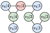
We provide an example in Figure 1 to show how the upper bounds are calculated and rules are used. Figure 1 shows a subgraph of G induced by the candidate set C = {v1, v2, · · · , v8}, i.e., G[C], of a 4-plex S, where vi|t identifies vertex vi ∈ C with δk (S, vi) = t. For simplification, we hide the 4-plex S and only depict the candidate vertices.
Suppose we sequentially color vertices v1, v2, · · · , v8 under the constraint that adjacent vertices cannot be in the same color, C can be partitioned into 3 independent sets, I1 = {v1, v2, v3}, I2 = {v4, v5, v6, v8} and I3 = {v7}, as indicated by the colors of the vertices. The GCB of ω4(G, S) is |S| + ∑3i=1 min{|Ii|, 4} = |S| + 3 + 4 + 1 = |S| + 8. The TISUB of ω4(G, S) is |S| + ∑3i=1 TISUB(Ii, S) = |S| + 3 + 2 + 1 = |S| + 6.
Then, let us use Rule 1 to make independent set I1 contain more vertices. For I1, since TISUB(I1, S) = 3, there is only one loose vertex v1 in I1. By applying Rule 1, we can add vertices v6 and v7 to I1 without increasing the upper bound of ω4(G[S ∪ I1], S), since there are only 3 loose or conflict vertices, i.e., v1, v6, v7, in I1 ∪ {v6, v7}. After the operation, C is partitioned into two sets, I5 = I1 ∪ {v6, v7} and I6 = {v4, v5, v8}. The new upper bound of ω4(G, S) is |S| +TISUB(I5, S) +TISUB(I6, S) = |S| +3+1 = |S| +4.
Finally, let us use Rule 2 to further make set I5 contain more vertices. According to Rule 2, all vertices in I6 can be added to I5 without increasing the upper bound of ω4(G[S ∪ I5], S). After the operation, the final RelaxGCB of ω4(G, S) is |S| + TISUB(I5, S) = |S| + 3.
3.4 The RelaxColoring Algorithm
The RelaxColoring algorithm for calculating the RelaxGCB is summarized in Algorithm 1. The algorithm first uses |S| to initialize the upper bound UB (line 1), and then repeatedly uses the TryColor() function to extract a subset I ⊆ C and calculate the upper bound on the number of vertices that I can provide for S, i.e., ub (line 3) until C = ∅ (line 2). After each execution of function TryColor(), the candidate set C and upper bound UB are both updated (line 4).
Function TryColor() is summarized in Algorithm 2, which first finds a maximal independent set I ⊆ C (lines 1-3) and calculates its TISUB (line 4). Then, the algorithm initializes
Algorithm 1: RelaxColoring(G, k, S, C)
Input: A graph G = (V, E), an integer k, the current partial k-plex S, the candidate set C Output: RelaxGCB of ωk(G, S) 1 initialize the upper bound UB ← |S|; 2 while C ̸= ∅ do 3 {I, ub} ←TryColor(G, k, S,C); 4 C ←C\I, UB ←UB +ub; 5 return UB;Algorithm 2: TryColor(G, k, S, C)
Input: A graph G = (V, E), an integer k, the current partial k-plex S, the candidate set C Output: A vertex set I, an upper bound ub of the number of vertices that I can provide for S 1 initialize I ← ∅; 2 for each vertex v ∈ C do 3 if N(v) ∩ I = ∅ then I ← I ∪ {v}; 4 ub ←TISUB(I, S); 5 initialize the set of loose or conflict vertices LC ← {v ∈ I|δk (S, v) > ub}; 6 if |LC| < ub then 7 for each vertex v ∈ C\I do 8 CV ← {v} ∪ {N(v) ∩ I\LC}; 9 if |LC| + |CV | ≤ ub then 10 I ← I ∪ {v}; 11 LC ← LC ∪ CV ; 12 if |LC| = ub then break; 13 for each vertex v ∈ C\I ∧ δk (S, v) < ub do 14 if |N(v) ∩ I| ≤ ub - δk (S, v) then 15 I ← I ∪ {v}; 16 return {I, ub};the set of loose or conflict vertices LC (line 5) and tries to add as many vertices as possible to I according to Rule 1 (lines 6-12). Once trying to add each vertex v, the algorithm uses CV to denote the extra conflict vertices caused by adding v to I (line 8). Since I is a maximal independent set in C, adding any vertex v to I increases at least one conflict vertices, i.e., v itself (line 8). Thus, the utilization of Rule 1 can be terminated when |LC| ≥ ub (lines 6 and 12). Finally, the algorithm applies Rule 2 to further add vertices to I (lines 1315). Since for each vertex v ∈ C\I, |N(v) ∩ I| > 0 holds, only vertex v ∈ C\I with δk (S, v) < ub can be added to I according to Rule 2 (line 13).
The time complexities of RelaxColoring algorithm and TryColor function are O(|C|2 × T ) and O(|C| × T ), respectively, where O(T) is the time complexity of the intersection operation between N(v) and I (or I\LC) used in lines 3, 8, and 14 in Algorithm 2. Actually, O(T ) is bounded by O(|V |) and much smaller than O(|V |) with the bitset encoding [Segundo et al., 2011].
Algorithm 3: SelectPartition(G, k, S, C)
Input: A graph G = (V, E), an integer k, the current partial k-plex S, the candidate set C Output: A vertex set I, an upper bound ub of the number of vertices that I can provide for S 1 initialize dise∗ ← 0, ub∗ ← 0, I ∗ ← ∅; 2 for each vertex v ∈ S ∧ δk (S, v) > 0 do 3 I ← C\N(v); 4 ub ←min{|I|, δk (S, v)}; 5 if |I|/ub > dise∗ ∨ (|I|/ub = dise∗ ∧ |I| > |I ∗ |) then dise∗ ← |I|/ub, ub∗ ← ub, I ∗ ← I ; 6 return {I ∗ , ub∗ };4 The RelaxPUB Bound
Motivated by the complementarity of the coloring-based and partition-based upper bounds, we propose to combine RelaxGCB with the newest PUB, DisePUB [Jiang et al., 2023], and propose a better and generic upper bound for MKP. In this section, we first introduce DisePUB, then provide two examples to illustrate the complementarity of the coloringbased and partition-based upper bounds, and finally present our new upper bound, RelaxPUB.
4.1 Revisiting DisePUB
Given a growing partial k-plex S and the corresponding candidate set C, for each vertex v ∈ S, DisePUB claims that a subset I ⊆ C can provide at most min{|I |, δk (S, v)} vertices for S if N(v)∩I = ∅. Given a vertex v ∈ S, let I = C\N(v) and ub = min{|I|, δk (S, v)}, DisePUB defines a metric for I, i.e., dise(I) = |I|/ub, to evaluate the extraction of vertex set I. The larger the value of dise(I), the more vertices that can be extracted from C and the fewer increments on the upper bound of ωk(G, S).
In each step, DisePUB traverses each vertex v ∈ S with δk (S, v) > 0 and selects the corresponding set I = C\N(v) with the largest value of dise(I). Ties are broken by preferring larger extractions. We use function SelectPartition() to describe the selection, which is shown in Algorithm 3. Then, DisePUB extracts C\N(v) from C and increases the upper bound of ωk(G, S) by min{|C\N(v)|, δk (S, v)}.
DisePUB repeats the above process until vertices remaining in C are adjacent to all vertices in S. DisePUB denotes the set of remaining vertices in C as π0 and finally increases the upper bound of ωk(G, S) by |π0|.
4.2 Complementarity of GCB and PUB
To better illustrate the complementarity of the coloring-based and partition-based upper bounds (i.e., GCB and PUB), we provide two examples in Figure 2, where the growing 2-plex S contains only one vertex v0 and its corresponding candidate set C = {v1, v2, v3, v4, v5}.
In Figure 2(a), the GCB is tighter than the PUB. The vertices in C are all adjacent to v0, which means the vertices in C are all in π0. Thus, the PUB is |S|+|π0| = 6. While by coloring the vertices in C, it can be partitioned into 2 independent sets I1 = {v1, v2, v3, v5} and I2 = {v4}, and the GCB is
Algorithm 4: SelectUB(G, k, S, C)
Input: A graph G = (V, E), an integer k, the current partial k-plex S, the candidate set C Output: RelaxPUB of ωk(G, S) 1 initialize the upper bound UB ← |S|; 2 while C ̸= ∅ do 3 {IC, ubC} ←TryColor(G, k, S,C); 4 {IP , ubP} ←SelectPartition(G, k, S,C); 5 if |IC|/ubC > |IP |/ubP ∨ (|IC|/ubC = |IP |/ubP ∧ |IC| > |IP |) then 6 C ← C\IC , UB ← UB + ubC ; 7 else 8 C ← C\IP , UB ← UB + ubP ; 9 return UB;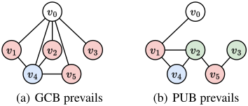
|S| + ∑2i=1 min{|Ii|, 2} = 4. In contrast, the PUB is tighter than the GCB in Figure 2(b), where C can be partitioned into 3 independent sets I1 = {v1, v5}, I2 = {v2, v3}, and I3 = {v4}. Thus, the GCB is |S| + ∑3i=1 min{|Ii|, 2} = 6. While vertices in C except v1 are non-adjacent to v0, π0 = {v1}, thus the PUB is |S| + |π0| + δ2 (S, v0) = 3.
4.3 Combining RelaxGCB and DisePUB
Both RelaxGCB and DisePUB extract a subset from C and accumulate the upper bound of ωk(G, S). The dise metric in DisePUB can also be used for the vertex set returned by TryColor(). RelaxPUB combines RelaxGCB and DisePUB by using them to select a promising extraction in each step.
We propose an algorithm called SelectUB for calculating the RelaxPUB of ωk(G, S), which is presented in Algorithm 4. The algorithm calls TryColor() and SelectPartition() in each step and figures out whose returned vertex set is better according to the dise metric. Ties are broken by preferring larger extraction. Once a better extraction is selected, The algorithm updates the candidate set C and accumulates the upper bound of ωk(G, S).
The time complexities of functions TryColor() and SelectPartition() are O(|C| × T) and O(|C| × |S|) [Jiang et al., 2023], respectively, where O(T ) is much smaller than O(|V |) as referred to Section 3.4. The time complexity of the SelectUB algorithm is O(|C|2 × (|S| + T )).
5 Experimental Results
This section presents experiments to evaluate the performance of RelaxGCB and RelaxPUB. Baselines contain SOTA BnB algorithms with GCB and PUB, i.e., Maplex [Zhou et al., 2021], kPlexS [Chang et al., 2022], DiseMKP [Jiang et al., 2023], an improvement version of KpLeX [Jiang et al., 2021], and KPLEX [Wang et al., 2023b]. We replace the original bounds in these baselines with RelaxGCB and RelaxPUB, conducting eight new BnB algorithms. Moreover, the recent kplexT algorithm [Chang and Yao, 2024] is also considered as a baseline, which does not contain GCB or PUB, and we compare it with our RelaxPUB-based algorithms.
5.1 Experimental Setup
All the algorithms 1 were implemented in C++ and run on a server using an AMD EPYC 7H12 CPU, running Ubuntu 18.04 Linux operation system. We test the algorithms on two public benchmarks that are widely used in the literature of the baselines, the 2nd DIMACS benchmark 2 that contains 80 (almost dense) graphs with up to 4,000 vertices and densities ranging from 0.03 to 0.99, and the Real-world benchmark 3 that contains 139 real-world sparse graphs from the Network Data Repository [Rossi and Ahmed, 2015].
We choose the two datasets because the 2nd DIMACS benchmark is also widely used to evaluate MCP, one of the most closely related problems to MKP, and the Real-world benchmark is widely used for analyzing various complex networks, one of the most important application areas of MKP. Moreover, the structures of the two benchmarks are distinct, helping evaluate the robustness of the algorithms.
For each graph, we generate 8 MKP instances with k ∈ {2, 3, 4, 5, 6, 7, 10, 15}, and set the cut-off time to 1,800 seconds per instance, following the settings of the baselines.
5.2 Performance Evaluation
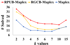
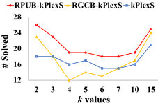
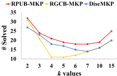
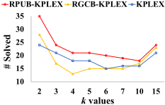
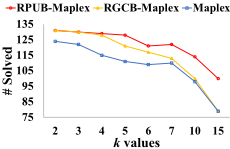
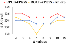
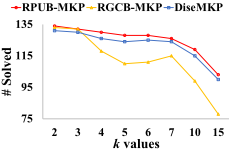
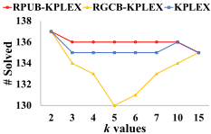
The comparison results between the algorithms with RelaxGCB and RelaxPUB (RGCB and RPUB in short) and the baselines in dense 2nd DIMACS and sparse Real-world benchmarks are summarized in Figures 3 and 4, respectively. The results are expressed by the number of MKP instances solved by each algorithm within the cut-off time for different k values. Note that Maplex only contains the GCB, and the other three baselines only contain the PUB. 1) From (a) of the two figures, one can observe that our RelaxGCB significantly outperforms GCB. 2) From (b) to (d) of the two figures, one can observe that RelaxGCB is complementary to PUB. 3) From all the figures, one can observe that our RelaxPUB makes full use of the complementarity of RelaxGCB and PUB, and significantly improves all the baselines in solving both dense and massive sparse graphs over diverse k values, indicating its dominant performance over the SOTA baselines, excellent generalization over different graphs, and strong robustness over diverse k values.
Following the convention of the baselines, we also present detailed results of the baselines and their improvements with RelaxPUB in solving 30 representative 2nd DIMACS and Real-world instances with k = 2, 3, 6, 10, 15 in Table 1. We report their running times in seconds (column Time), the sizes
1 Source code: https://github.com/JHL-HUST/RelaxPUB
2 http://archive.dimacs.rutgers.edu/pub/challenge/graph/ benchmarks/clique/
3 http://lcs.ios.ac.cn/%7Ecaisw/Resource/realworld%20 graphs.tar.gz
- (a) Comparison with Maplex
- (b) Comparison with kPlexS
- (c) Comparisons with DiseMKP
(d) Comparison with KPLEX
- (a) Comparison with Maplex
- (b) Comparison with kPlexS
- (c) Comparison with DiseMKP
- (d) Comparison with KPLEX
| k | Instance | RelaxPUB-Maplex | Maplex | RelaxPUB-kPlexS | kPlexS | RelaxPUB-MKP | DiseMKP | RelaxPUB-KPLEX | KPLEX | |||||||||||||||
|---|---|---|---|---|---|---|---|---|---|---|---|---|---|---|---|---|---|---|---|---|---|---|---|---|
| Tree | Time | Percent | Tree | Time | Tree | Time | Percent | Tree | Time | Tree | Time | Percent | Tree | Time | Tree | Time | Percent | Tree | Time | |||||
| 2 | brock200-3 brock200-4 C125.9 keller4 | 9.432 24.99 88.36 | 10.06 | 790.8 | 107.8 | 8.343 | 292.0 | 49.9% | 52.35 | 1,615 | 7.393 | 21.93 | 46.2% | 85.88 | 26.06 | 27.43 | 34.63 | 79.8% | 225.2 | 80.52 | ||||
| 30.07 | 49.7% 50.2% | 4015 | 576.9 - | 23.84 | 695.8 | 49.7% | - | - | 12.60 | 47.20 | 49.8% | 279.6 | 103.1 | 68.81 | 84.81 | 78.8% | 780.2 | 250.0 | ||||||
| 186.3 | 66.3% | - | 24.56 | 162.8 | 71.8% | - | - | 15.32 | 69.65 | 70.5% | - | - | 29.61 | 37.93 88.0% | - | - | ||||||||
| 3.715 | 4.015 | 46.1% | 1273 | 182.3 | 3.961 | 87.18 | 44.3% | 92.45 | 1,238 | 2.666 | 8.016 | 42.0% | 69.11 | 21.15 | 19.29 | 17.38 | 79.6% | 562.6 | 105.3 | |||||
| san200-0-9-1 | 0.004 | 0.051 | 93.0% | - | - | 0.024 | 0.660 | 94.8% | - | - | 0.003 | 0.105 | 95.2% | - | - | 0.057 | 0.619 | 98.4% | 64.21 | 27.33 | ||||
| sanr200-0-7 | 96.72 | 135.8 | 49.5% | - | - | 66.05 | 1,656 | 51.5% | - | - | 40.59 | 153.0 | 49.9% | 1130 | 475.4 | 171.7 | 206.6 | 79.5% | 2681 | 752.0 | ||||
| socfb-Duke14 | 0.579 | 2.313 | 78.7% | 195.6 | 45.05 | 0.110 | 4.397 | 85.8% | 1.046 | 36.58 | 0.213 | 2.121 | 83.4% | 243.6 | 154.5 | 0.281 | 2.403 | 94.3% | 1.598 | 2.957 | ||||
| socfb-UF | 0.253 | 3.217 | 88.3% | - | - | 0.094 | 2.012 | 93.2% | 0.190 | 3.310 | 0.069 | 2.800 | 91.5% | 413.1 | 299.3 | 0.107 | 1.741 | 91.9% | 0.234 | 1.850 | ||||
| socfb-Uillinois | 0.229 | 7.991 | 89.3% | - | - | 0.022 | 2.224 | 92.8% | 0.023 | 2.628 | 0.168 | 4.138 | 81.0% | 18.33 | 13.05 | 0.024 | 1.774 | 85.8% | 0.027 | 1.845 | ||||
| 3 | hamming6-2 MANN-a81 p-hat300-2 socfb-UF socfb-Indiana soc-flixster | 393.2 | 399.6 | - | - | 204.4 | 349.2 | 49.8% | - | - | 137.4 | 234.1 | 49.1% | 304.6 | 197.0 | 136.2 | 60.2% | 1157 | 203.3 | |||||
| 0.001 | 0.001 | 57.6% 100% | - | - | 0.001 | 534.9 | 96.3% | 0.001 | 556.1 | 0.001 | 62.67 | 98.3% | 826.6 0.003 | 63.61 | 0.004 | 568.4 | 98.9% | 0.406 | 605.2 | |||||
| 174.7 | 340.9 | 57.0% | - | - | 123.6 | 1,565 | 57.2% | - | - | 36.99 | 200.0 | 59.2% | - | - | 401.9 | 470.9 | 75.3% | 1293 | 529.0 | |||||
| 82.41 | 254.3 | 87.3% | - | - | 0.094 | 1.975 | 82.1% | 0.324 | 4.172 | 6.950 | 40.60 | 86.7% | 440.6 | 413.4 | 0.067 | 1.877 | 89.4% | 0.079 | 2.104 | |||||
| 2.437 | 8.069 | 89.1% | 1002 | 308.6 | 0.007 | 1.722 | 82.8% | 0.008 | 1.879 | 1.110 | 7.302 | 84.9% | 587.8 | 391.5 | 0.006 | 1.436 | 89.9% | 0.006 | 1.708 | |||||
| 8.732 | 20.00 | 74.6% | - | - | 0.725 | 8.152 | 73.5% | 7.394 | 110.5 | 2.084 | 13.15 | 76.2% | 118.0 | 85.04 | 0.280 | 3.982 | 84.7% | 0.470 | 5.674 | |||||
| soc-lastfm | 1.384 | 6.018 | 54.8% | 78.33 | 29.91 | 0.327 | 17.86 | 60.2% | 0.785 | 43.87 | 0.729 | 9.750 | 52.4% | 7.163 | 10.26 | 1.549 | 53.88 | 77.5% | 2.819 | 95.76 | ||||
| soc-slashdot | 1.607 | 1.922 | 74.2% | 2461 | 289.2 | 0.095 | 0.715 | 72.3% | 0.299 | 2.825 | 0.245 | 0.910 | 76.9% | 7.847 | 4.577 | 0.096 | 0.829 | 82.4% | 0.131 | 0.766 | ||||
| tech-WHOIS | 24.96 | 72.23 | 85.3% | - | - | 0.049 | 0.451 | 84.4% | 0.134 | 1.647 | 0.384 | 2.514 | 89.8% | 6.996 | 6.043 | 0.028 | 0.279 | 90.9% | 0.034 | 0.483 | ||||
| 6 | c-fat200-1 | 0.001 | 0.001 | 92.8% | 0.001 | 0.001 | 0.001 | 80.6% | 0.001 | 0.002 | 0.002 | 0.014 | 82.9% | 0.002 | 0.018 | 0.001 | 66.0% | 0.001 | 0.001 | |||||
| san200-0-7-1 | 0.001 | 0.017 | 95.9% | 0.003 - | - | 0.001 | 0.040 | 93.3% | 3.163 | 4.928 | 0.001 | 0.037 | 93.7% | 0.329 | 0.177 | 0.001 0.001 | 0.043 | 87.1% | - | - | ||||
| san200-0-7-2 | 0.001 | 0.012 | 80.1% | 11.99 | 6.417 | 0.004 | 0.156 | 70.4% | - | - | 0.005 | 0.066 | 68.8% | - | - | 0.122 | 81.8% | - | - | |||||
| socfb-Berkeley13 | 0.078 | 1.514 | 94.4% | 1780 | 249.5 | 0.001 | 0.890 | 50.0% | 0.001 | 0.905 | 0.244 | 1.890 | 90.4% | 4.509 | 4.586 | 0.002 0.001 | 0.828 | 28.2% | 0.001 | 0.867 | ||||
| socfb-MIT | 0.189 | 0.591 | 78.4% | 15876 | 1684 | 0.002 | 0.317 | 70.7% | 0.002 | 0.319 | 0.041 | 0.523 | 91.4% | 2.220 | 1.764 | 0.002 | 0.271 | 57.0% | 0.002 | 0.340 | ||||
| soc-gowalla | 12.45 | 11.61 | 54.2% | 779.5 | 120.1 | 0.003 | 0.430 | 63.4% | 0.005 | 0.572 | 6.042 | 16.65 | 53.1% | 59.68 | 43.12 | 0.004 | 0.199 | 69.3% | 0.004 | 0.242 | ||||
| 10 | bio-dmela | 1.245 | 14.64 | 39.1% | - | - | 0.004 | 0.067 | 48.7% | 0.007 | 0.076 | 0.085 | 0.113 | 30.9% | 4.615 | 0.221 | 0.019 | 0.037 | 57.1% | 0.030 | 0.038 | |||
| ia-enron-large | 5.779 | 4.850 | 55.4% | 156.3 | 24.10 | 0.001 | 0.103 | 76.3% | 0.001 | 0.115 | 14.80 | 24.89 | 39.6% | 266.7 | 178.1 | 0.064 | 72.1% | 0.002 | 0.065 0.068 | |||||
| tech-RL-caida | 0.662 | 0.803 | 46.9% | 18.52 | 4.693 | 0.001 | 0.251 | 65.9% | 0.001 | 0.258 | 0.017 | 0.363 | 73.2% | 1.160 | 0.500 | 0.002 0.001 | 0.067 | 83.3% 0.001 | ||||||
| 15 | C125-9 | 152.7 | 507.5 | 79.6% | - | - | 5.460 | 30.22 | 70.4% | 12.21 | 96.15 | 2.712 | 16.10 | 82.6% | 7.771 | 22.62 | 1.194 | 5.414 | 83.5% | 17.47 | 40.32 | |||
| bio-diseasome | 0.234 | 0.145 | 80.1% | 1011 | 169.0 | 0.001 | 0.001 | 81.3% | 0.001 | 0.001 | 0.055 | 0.024 | 57.7% | 80.71 | 2.321 | 0.000 | 0.000 | 0.000 | 0.001 | |||||
| socfb-uci-uni | 22.61 | 107.5 | 47.9% | - | - | 0.019 | 49.43 | 58.1% | 0.517 | 53.96 | 26.93 | 295.4 | 35.6% | - | - | 0.185 | 62.7% | 6.775 | 100% | 1.096 9.322 | ||||
(a) On DIMACS2 benchmark (b) On Real-world benchmark Figure 5: Comparisons of our RelaxPUB algorithms and kplexT.
of their entire search trees in 105 (column Tree) to solve the instances, and the percentage of the number of times RelaxGCB is selected and outperforms the DisePUB in RelaxPUB (column Percent). Better results are highlighted in bold, and symbol '-' means the algorithm cannot solve the instance within the cut-off time.
The results show that for each pair of tested algorithms, our new upper bounds can help the baseline algorithm prune significantly more branches, reducing its search tree sizes by several orders of magnitude for instances that both can solve within the cut-off time. There are also many instances that the baseline algorithms cannot solve within the cut-off time, while the algorithms with our upper bounds can solve with few branches and much less calculation time. Moreover, we can observe that RelaxGCB contributes a lot in solving these instances, indicating again the complementarity of RelaxGCB and DisePUB.
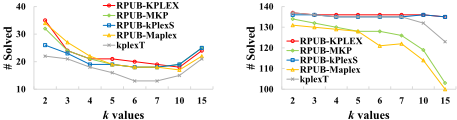
Moreover, we compare our RelaxPUB algorithms with the kplexT algorithm. The results are shown in Figure 5. We can observe that in Real-world benchmark, RelaxPUBkPlexS and RelaxPUB-KPLEX show better performance than kplexT, and in DIMACS2 benchmark, kplexT shows the worst performance, indicating that our method indeed leads to SOTA BnB algorithms for MKP. By the way, kplexT mentioned that the PUB may be used to improve it in its future work [Chang and Yao, 2024], indicating that our method indeed improves a general and popular technique.
5.3 Ablation Study
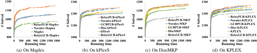
The ablation studies contain two parts. The first part is to evaluate the effectiveness of the proposed TISUB and the two rules (see Lemmas 1, 2, and 3) in our proposed upper bounds. For the kPlexS, DiseMKP, and KPLEX baselines having the PUB, we generate a "Norules" variant, which uses our RelaxPUB without Rules 1 and 2, and a "GCBPUB" variant, which uses our RelaxPUB and replaces its RelaxGCB with the GCB in Maplex. Moreover, since the kPlexS and KPLEX algorithms use the previous PUB proposed in [Jiang et al., 2021], we apply the newest DisePUB to them and obtain two variants: Dise-kPlexS and Dise-KPLEX. For the Maplex baseline that is only based on GCB, its "Norules" variant uses our RelaxGCB without Rules 1 and 2.
We perform four groups of ablation studies based on each baseline over all the 1,752 instances, as summarized in Figure 6. The results are expressed by the variation in the number of solved instances for each algorithm over the running time (in seconds). The results show that the "GCBPUB" variants are better than the baselines, indicating that combining coloring-based and partition-based upper bounds by the mechanism in RelaxPUB can make use of their complementarity. The "Norules" variants are better than the "GCBPUB" variants, indicating that TISUB is a significant improvement over GCB. The new algorithms with RelaxPUB are better than the "Norules" variants, indicating that our proposed two rules can further improve TISUB. Moreover, DisePUB can hardly improve kPlexS and KPLEX, indicating that the improvements of the RelaxPUB series over the baselines originate from RelaxGCB rather than using the newest DisePUB.
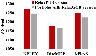
The second part is to evaluate the effectiveness of the combination scheme designed in RelaxPUB. In this part, we compare each of the RelaxPUB algorithms with the portfolio consist of the corresponding baseline and its RelaxGCB algorithm. For example for the KPLEX algorithm, the portfolio version outputs the better result found by KPLEX and RelaxGCB-KPLEX, i.e., if any of KPLEX and RelaxGCBKPLEX solve the solution, the portfolio solves the solution. The comparison results on all the 1,752 tested instances are shown in Figure 7. Note that we only perform on the baselines with PUB, i.e., KPLEX, DiseMKP, and kPlexS. The results show that the RelaxPUB algorithms can solve more instances than the portfolio ones, indicating the advantages of the combination scheme in RelaxPUB, which can make fully use of the complementarity of RelaxGCB and PUB.
6 Conclusion
We proposed two new upper bounds for the Maximum kplex Problem (MKP), termed RelaxGCB and RelaxPUB. RelaxGCB considers the connectivity between vertices more thoroughly and relaxes the restrictive independent set structure to contain more vertices without increasing the upper bound. Provided theoretical proof indicates that RelaxGCB is strictly better than the previous graph color bound (GCB). RelaxPUB further combines RelaxGCB and an advanced partition-based upper bound in a novel way, making fully use of their complementarity. We replaced the GCB in Maplex and the partition-based upper bounds in kPlexS, DiseMKP, and KPLEX with RelaxGCB and RelaxPUB, respectively, producing eight new BnB MKP algorithms. Experiments on both dense and sparse graph datasets show that RelaxGCB significantly outperforms GCB, and RelaxPUB exhibits clearly priority over the baselines and exhibits excellent robustness over various k values and high generalization capability over different graphs and algorithms.
RelaxGCB contains ideas of enhancing coloring-based upper bounds in relaxation clique problems, and RelaxPUB contains ideas of combining complementary upper bounds. We believe our methods can be applied for improving BnB algorithms of other relaxation clique problems.
Contribution Statement
The first two authors, Jiongzhi Zheng and Mingming Jin, contributed equally.
@inproceedings{ijcai2025p1002,
  title     = {Exact Algorithms with New Upper Bounds for the Maximum k-plex Problem},
  author    = {Zheng, Jiongzhi and Jin, Mingming and He, Kun},
  booktitle = {Proceedings of the Thirty-Fourth International Joint Conference on
               Artificial Intelligence, {IJCAI-25}},
  publisher = {International Joint Conferences on Artificial Intelligence Organization},
  editor    = {James Kwok},
  pages     = {9014--9021},
  year      = {2025},
  month     = {8},
  note      = {Main Track},
  doi       = {10.24963/ijcai.2025/1002},
  url       = {https://doi.org/10.24963/ijcai.2025/1002},
}
TY - CPAPER TI - Exact Algorithms with New Upper Bounds for the Maximum k-plex Problem AU - Zheng, Jiongzhi AU - Jin, Mingming AU - He, Kun T2 - Proceedings of the Thirty-Fourth International Joint Conference on Artificial Intelligence, IJCAI-25 PB - International Joint Conferences on Artificial Intelligence Organization PY - 2025 SP - 9014 EP - 9021 DO - 10.24963/ijcai.2025/1002 UR - https://doi.org/10.24963/ijcai.2025/1002 ER -Copied
Machine-readable versions of this paper, for tools and AI agents:





