
Non-collective Calibrating Strategy for Time Series Forecasting
Proceedings of the Thirty-Fourth International Joint Conference on Artificial Intelligence. Main Track. Pages 3335-3343.
https://doi.org/10.24963/ijcai.2025/371
Keywords
- Data Mining: DM: Applications
- Machine Learning: ML: Deep learning architectures
- Machine Learning: ML: Multi-task and transfer learning
- Data Mining: DM: Mining spatial and/or temporal data
Abstract
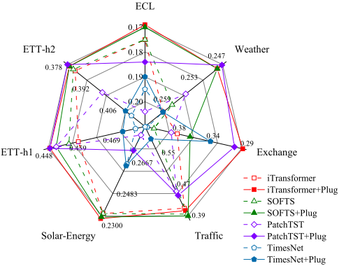
Deep learning-based approaches have demonstrated significant advancements in time series forecasting. Despite these ongoing developments, the complex dynamics of time series make it challenging to establish the rule of thumb for designing the golden model architecture. In this study, we argue that refining existing advanced models through a universal calibrating strategy can deliver substantial benefits with minimal resource costs, as opposed to elaborating and training a new model from scratch. We first identify a multi-target learning conflict in the calibrating process, which arises when optimizing variables across time steps, leading to the underutilization of the model's learning capabilities. To address this issue, we propose an innovative calibrating strategy called Socket+Plug (SoP). This approach retains an exclusive optimizer and early-stopping monitor for each predicted target within each Plug while keeping the fully trained Socket backbone frozen. The model-agnostic nature of SoP allows it to directly calibrate the performance of any trained deep forecasting models, regardless of their specific architectures. Extensive experiments on various time series benchmarks and a spatio-temporal meteorological ERA5 dataset demonstrate the effectiveness of SoP, achieving up to a 22% improvement even when employing a simple MLP as the Plug (highlighted in Figure 1).
- [Alibaba Group, 2023] Alibaba Group. The First World Sci- ence and Intelligence Competition: Atmospheric Science Track -East China AI Medium-Range Weather Forecast- ing Competition. https://tianchi.aliyun.com/competition/ entrance/532111/information, 2023. Link
- [Ba et al., 2016] Lei Jimmy Ba, Jamie Ryan Kiros, and Geoffrey E. Hinton. Layer normalization. CoRR, abs/1607.06450, 2016.
- [Berta et al., 2024] Eugene Berta, Francis Bach, and Michael Jordan. Classifier calibration with roc-regularized isotonic regression. In International Conference on Artifi- cial Intelligence and Statistics, pages 1972-1980. PMLR, 2024.
- [Bi et al., 2023] Kaifeng Bi, Lingxi Xie, Hengheng Zhang, Xin Chen, Xiaotao Gu, and Qi Tian. Accurate medium- range global weather forecasting with 3d neural networks. Nat., 619(7970):533-538, 2023.
- [Borovykh et al., 2017] Anastasia Borovykh, Sander Bohte, and Cornelis W Oosterlee. Conditional time series fore- casting with convolutional neural networks. arXiv, 2017.
- [Chen et al., 2023a] Lei Chen, Xiaohui Zhong, Feng Zhang, Yuan Cheng, Yinghui Xu, Yuan Qi, and Hao Li. FuXi: A cascade machine learning forecasting system for 15-day global weather forecast. npj Climate and Atmospheric Sci- ence, 6(1):190, 2023.
- [Chen et al., 2023b] Si-An Chen, Chun-Liang Li, Sercan Ö. Arik, Nathanael C. Yoder, and Tomas Pfister. TSMixer: An all-mlp architecture for time series forecast-ing. Trans. Mach. Learn. Res., 2023, 2023.
- [Deng et al., 2022] Jinliang Deng, Xiusi Chen, Renhe Jiang, Xuan Song, and Ivor W Tsang. A multi-view multi-task learning framework for multi-variate time series forecast- ing. IEEE Transactions on Knowledge and Data Engineer- ing, 35(8):7665-7680, 2022.
- [Deng et al., 2024a] Jinliang Deng, Xiusi Chen, Renhe Jiang, Du Yin, Yi Yang, Xuan Song, and Ivor W. Tsang. Disentangling structured components: Towards adaptive, interpretable and scalable time series forecasting. IEEE Transactions on Knowledge and Data Engineering, 2024.
- [Deng et al., 2024b] Jinliang Deng, Feiyang Ye, Du Yin, Xuan Song, Ivor Tsang, and Hui Xiong. Parsimony or capability? decomposition delivers both in long-term time series forecasting. Advances in Neural Information Pro- cessing Systems, 37:66687-66712, 2024.
- [Han et al., 2024] Lu Han, Xu-Yang Chen, Han-Jia Ye, and De-Chuan Zhan. SOFTS: efficient multivariate time series forecasting with series-core fusion. CoRR, abs/2404.14197, 2024.
- [Hendrycks and Gimpel, 2016] Dan Hendrycks and Kevin Gimpel. Gaussian error linear units (gelus). arXiv preprint arXiv:1606.08415, 2016.
- [Huang et al., 2023] Yulong Huang, Yang Zhang, Qifan Wang, Chenxu Wang, and Fuli Feng. Prediction then cor- rection: An abductive prediction correction method for se- quential recommendation. In SIGIR, pages 2272-2276. ACM, 2023.
- [Kuleshov et al., 2018] Volodymyr Kuleshov, Nathan Fen- ner, and Stefano Ermon. Accurate uncertainties for deep learning using calibrated regression. In ICML, volume 80 of Proceedings of Machine Learning Research, pages 2801-2809. PMLR, 2018.
- [Lai et al., 2018] Guokun Lai, Wei-Cheng Chang, Yiming Yang, and Hanxiao Liu. Modeling long-and short-term temporal patterns with deep neural networks. In SIGIR, pages 95-104. ACM, 2018.
- [Liu et al., 2021] H Liu, L Dong, R Yan, X Zhang, C Guo, S Liang, J Tu, X Feng, and X Wang. Evaluation of near- surface wind speed climatology and long-term trend over china's mainland region based on ERA5 reanalysis. Cli- matic and Environmental Research, 26(3):299-311, 2021.
- [Liu et al., 2024a] Xu Liu, Junfeng Hu, Yuan Li, Shizhe Diao, Yuxuan Liang, Bryan Hooi, and Roger Zimmer- mann. Unitime: A language-empowered unified model for cross-domain time series forecasting. In Proceedings of the ACM Web Conference 2024, pages 4095-4106, 2024.
- [Liu et al., 2024b] Yong Liu, Tengge Hu, Haoran Zhang, Haixu Wu, Shiyu Wang, Lintao Ma, and Mingsheng Long. iTransformer: Inverted Transformers Are Effective for Time Series Forecasting. In ICLR, 2024.
- [Lu et al., 2018] Jie Lu, Junyu Xuan, Guangquan Zhang, and Xiangfeng Luo. Structural property-aware multilayer net- work embedding for latent factor analysis. Pattern Recog- nition, 76:228-241, 2018.
- [Lu et al., 2019] Jie Lu, Hua Zuo, and Guangquan Zhang. Fuzzy multiple-source transfer learning. IEEE Transac- tions on Fuzzy Systems, 28(12):3418-3431, 2019.
- [Nie et al., 2023] Yuqi Nie, Nam H. Nguyen, Phanwadee Sinthong, and Jayant Kalagnanam. A time series is worth 64 words: Long-term forecasting with transformers. In ICLR, 2023.
- [Platt and others, 1999] John Platt et al. Probabilistic outputs for support vector machines and comparisons to regular- ized likelihood methods. Advances in large margin classi- fiers, 10(3):61-74, 1999.
- [Platt, 2000] John C. Platt. Probabilistic outputs for support vector machines and comparisons to regularized likelihood methods. Advances in Large Margin Classifiers, 2000.
- [Qiu et al., 2024] Xiangfei Qiu, Jilin Hu, Lekui Zhou, Xingjian Wu, Junyang Du, Buang Zhang, Chenjuan Guo, Aoying Zhou, Christian S. Jensen, Zhenli Sheng, and Bin Yang. TFB: towards comprehensive and fair bench- marking of time series forecasting methods. VLDB, 17(9):2363-2377, 2024.
- [Ronneberger et al., 2015] Olaf Ronneberger, Philipp Fis- cher, and Thomas Brox. U-Net: Convolutional networks for biomedical image segmentation. In MICCAI, volume 9351 of Lecture Notes in Computer Science, pages 234- 241. Springer, 2015.
- [Sun et al., 2023] Chunlin Sun, Linyu Liu, and Xiaocheng Li. Predict-then-Calibrate: A New Perspective of Robust Contextual LP. In NeurIPS, 2023.
- [Tan et al., 2024] Mingtian Tan, Mike A Merrill, Vinayak Gupta, Tim Althoff, and Thomas Hartvigsen. Are lan- guage models actually useful for time series forecasting? In NeurIPS, 2024.
- [Wang et al., 2024] Yuxuan Wang, Haixu Wu, Jiaxiang Dong, Yong Liu, Mingsheng Long, and Jianmin Wang. Deep time series models: A comprehensive survey and benchmark. CoRR, abs/2407.13278, 2024.
- [Wen et al., 2023] Haomin Wen, Youfang Lin, Yutong Xia, Huaiyu Wan, Qingsong Wen, Roger Zimmermann, and Yuxuan Liang. Diffstg: Probabilistic spatio-temporal graph forecasting with denoising diffusion models. In Pro- ceedings of the 31st ACM International Conference on Ad- vances in Geographic Information Systems, pages 1-12, 2023.
- [Wu et al., 2023] Haixu Wu, Tengge Hu, Yong Liu, Hang Zhou, Jianmin Wang, and Mingsheng Long. TimesNet: Temporal 2d-variation modeling for general time series analysis. In ICLR. OpenReview.net, 2023.
- [Zeng et al., 2023] Ailing Zeng, Muxi Chen, Lei Zhang, and Qiang Xu. Are transformers effective for time series fore- casting? Proceedings of the AAAI Conference on Artificial Intelligence, 37(9):11121-11128, Jun. 2023.
- [Zhang et al., 2023] Rongtao Zhang, Xueling Ma, Weiping Ding, and Jianming Zhan. MAP-FCRNN: multi-step ahead prediction model using forecasting correction and RNN model with memory functions. Inf. Sci., 646:119382, 2023.
- [Zhang et al., 2024] Jiawen Zhang, Xumeng Wen, Zhenwei Zhang, Shun Zheng, Jia Li, and Jiang Bian. ProbTS: Benchmarking point and distributional forecasting across diverse prediction horizons. In NeurIPS, 2024.
- [Zhong et al., 2025] Siru Zhong, Weilin Ruan, Ming Jin, Huan Li, Qingsong Wen, and Yuxuan Liang. Time-vlm: Exploring multimodal vision-language models for aug- mented time series forecasting. In Proceedings of the 42nd International Conference on Machine Learning, 2025.
- [Zhou et al., 2022] Tian Zhou, Ziqing Ma, Qingsong Wen, Xue Wang, Liang Sun, and Rong Jin. FEDformer: Fre- quency enhanced decomposed transformer for long-term series forecasting. In ICML, volume 162 of Proceedings of Machine Learning Research, pages 27268-27286. PMLR, 2022.
References were extracted automatically from the PDF and may contain errors.
Full text extracted automatically from the PDF; figures, tables and equations may differ. The PDF is the version of record.
1 Introduction
Time series forecasting remains challenging due to the inherent diversity and complexity of the data, which are influenced by factors such as seasonal fluctuations, trends, and domainspecific patterns [Deng et al., 2024a]. To investigate the most effective deep learning architecture, researchers have endeavored from convolutional neural networks (CNNs) [Borovykh et al., 2017] and recurrent neural networks (RNNs) [Lai et al., 2018] to graph neural networks (GNNs) [Wen et al., 2023] and Transformers [Zhang et al., 2024]. However, empirical debates persist regarding the performance of these models in time series forecasting. For instance, some studies have revisited the argument that a properly designed simple multi-layer perceptron (MLP) can outperform advanced Transformer-based models [Zeng et al., 2023; Lu et al., 2018]. With SOTA models emerging almost daily, disagreements over performance can incur significant inefficiencies for decision-makers during model selection. Consider a scenario where a trained model is already performing effectively in a production environment, yet numerous novel SOTA models continue to emerge. Determining whether any of these newmodels has the potential to surpass the deployed model typically requires extensive trial-and-error experimentation. This raises a critical question: rather than exhaustively testing each new SOTA model, could the existing trained model be enhanced at minimal cost?
† Feng Hong and Yanwei Yu are corresponding authors.
In this study, we instead draw attention to harness trained time series forecasting methods rather than designing a new model from scratch. An intuitive solution involves calibrating time series predictions using prior knowledge, such as rulebased methods that apply exponential smoothing and filtering to reduce noise and constraint bounds. Despite their simplicity, such approaches demand rigorous domain knowledge, as improper handling can degrade performance. Motivated by the effectiveness of learning-based classification calibration [Platt, 2000], we would explore its potential in time series forecasting models.
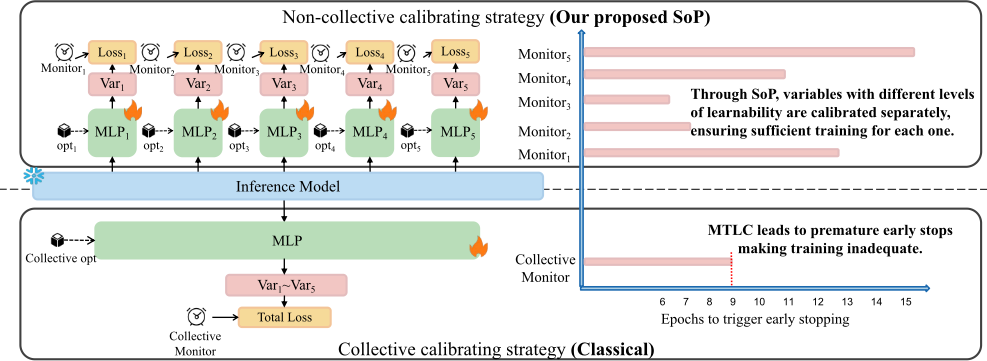
Classical calibrating typically involves keeping the fully trained model frozen while post-processing only the outputs of the forecasting models [Kuleshov et al., 2018]. Generally, this process calibrates the predictive bias across all target variables and prediction horizons simultaneously, a strategy we term as collective calibrating in this study. In contrast, when the calibrating process is applied separately to grouped or individual variables or prediction horizons, we introduce the term non-collective calibrating. To investigate the effect of these two strategies, we started by conducting a preliminary experiment, with the key discovery illustrated in Figure 2 and described as follows. Employing a classical collective calibrating strategy - where an additional MLP to be finetuned (illustrated in the bottom part of Figure 2) is attached to the existing trained inference model (represent by the blue rectangle)- we observed premature triggering (e.g., around 10 epochs) of the early-stopping monitor. Conversely, when the single MLP was split equally by the number of neurons into five smaller, independent MLPs denoted as MLP1 to MLP5, each dedicated to be finetuned for a single target variable and equipped with its own optimizer and early-stopping monitor (illustrated in the upper part of Figure 2), we observed significant variation in the early-stopping epochs across monitors. While some stopped in fewer than 10 epochs, others required substantially more epochs to achieve optimal performance on validation data.
Our heuristic hypothesis is that, due to varying levels of learnability across different targets, optimizing all variables simultaneously under the same objective loss function may fail to fully capture the unique distribution of each target variable - a phenomenon we refer to as multi-target learning conflict (MTLC).
To test the above hypothesis, we have conducted rigorous ablation study to compare the forecasting performance of the two strategies. Our findings support that the non-collective calibrating strategy outperforms its collective counterpart regarding generalization performance (referred to Table 2). We metaphorically term this approach the Socket+Plug strategy (SoP), where the well-trained inference model serves as a Socket, providing the fundamental shared predictive ability, while each additional module (e.g., MLP) as a Plug, tailored to its specific calibrating target. Extensive experiments further demonstrate that SoP can generally enhance the performance when existing deep forecasting models are taken as the Socket, as highlighted in Figure 1. We further investigated two specific forms of SoP: variable-wise SoP and step-wise SoP. Experimental results indicate that, under the same model architectures, both step-wise and variable-wise SoP exhibit similarly strong performance. It is worth noting that SoP leverages off-the-shelf Socket outputs without requiring any modifications to the Socket, making it easily combined with existing SOTA deep forecasting methods. Moreover, we applied SoP to the spatio-temporal meteorological forecasting task, utilizing Unet as the Socket. The experimental results validate its effectiveness, highlighting its potential for integration with advanced weather forecasting systems, such as PanGu [Bi et al., 2023] and FengWu [Chen et al., 2023a], thereby underscoring its applicability to real-world weather forecasting tasks. In summary, the key contributions of this study are summarized as follows:
- To our best knowledge, we are the first to identify and emphasize the detrimental impact of the MTLC phe-
nomenon in deep forecasting, which limits the learning potential of time series models. Specifically, we demonstrate that the traditional early-stopping mechanism in model training could fail to fully exploit the capabilities of these models.
- We propose SoP, a universal and model-agnostic calibrating strategy, developed to calibrate the performance of fully trained deep forecasting models with minimal design costs. By employing a dedicated optimizer and early-stopping monitor for each predicted target, SoP effectively mitigates the MTLC issue.
- We derive two specific forms of SoP, referred to as target-wise SoP, which include variable-wise SoP and step-wise SoP. Both demonstrate significantly better performance than classical collective calibrating and can be used as quick-start versions of SoP, eliminating the need to determine the Counts hyperparameter for the Plug.
- We conduct extensive experiments on seven time series benchmark datasets and the spatio-temporal ERA5 meteorological dataset, whose results demonstrate the effectiveness of SoP, achieving up to a 22% improvement in forecasting performance. This showcases its potential for advancing time series and spatio-temporal forecasting tasks.
2 Preliminaries
2.1 Definitions
Definition 1 (Time Series Forecasting). Given a historical observation series X = {x1, x2, . . . , xT } ∈ RN×T , which represents past T time steps and N variables, let X:,t denote the values of all variables at time step t, and Xn,: denote the values across all past time steps for variable n. Time series forecasting aims to learn a model f(·) that predicts the future values ¯ Y = f(X) = {xT+1, xT+2, . . . , xT+S} ∈ RN×S over the future S time steps, a.k.a., S prediction horizons.
Definition 2 (Collective & Non-collective calibrating). Traditional calibrating typically involves keeping the inference model frozen while re-training part of model layers collectively for all target variables across all prediction horizons. We define this type of calibrating as collective calibrating. In contrast, when the calibrating process is applied separately to grouped or even individual variables or prediction horizons, we denote this as non-collective calibrating. With these definitions, our proposed SoP strategy falls under non-collective calibrating.
Definition 3 (Optimized Plug & Plug Counts). When implementing SoP, one can decide how many variables or prediction horizons are optimized together as a group, each with its own optimizer and early-stopping monitor. We refer to each such group of variables or horizons as an Optimized Plug and the number of total optimized plugs is denoted as the Plug Counts. Specifically, for a prediction target Y ∈ RN×S : If n variables along the N-dimension form an optimized plug to predict Yplug ∈ Rn×S , SoP creates the plug counts as M = Nn . If s horizons along the S-dimension form an optimized plug to predict Yplug ∈ RN×s , SoP creates the plug counts as M = Ss . Two special remarks are derived as:
Remark 1. There are two types of target-wise SoP: when n = 1, M = N, it is referred to as the variable-wise SoP; and when s = 1, M = S, it is referred to as the step-wise SoP. Remark 2. When n = N and s = S, M = 1, in which case
SoP reduces to the classical collective calibrating strategy.
3 Methodology
To clarify the data flow in the model operation based on SoP, this section first introduces the model inference process given the input, followed by an explanation of the calibrating process of SoP. Without loss of generality and for clarity, we use a variable-wise SoP (where M = N, as described in Remark 1.) to illustrate the process.
3.1 Model Inference
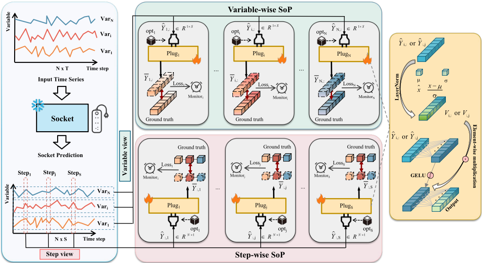
As shown in Figure 3, the proposed SoP strategy operates on the basis of two key components: the Socket and the Plug. The Socket is adopted to capture complex correlations among variables and deliver the high-quality foundational forecasts. To this end, it is recommended to harness a trained SOTA forecasting model, such as a Transformer-based variant, as the Socket. Given an input sample X ∈ RN×T , the Socket can preliminarily infer the prediction of the future sequence ˆ Y as follows:
The obtained ˆ Y is then divided into M groups along the dimension of variables or horizons. Specifically, in the case of variable-wise SoP, ˆ Y is divided into N groups based on each variable index i, forming ˆ Yi,: ∈ RS . Each ˆ Yi,: undergoes layer normalization to produce the normalized values Vi,:, a technique demonstrated to improve the stability of the training convergence [Ba et al., 2016], and then is processed by a Plugi for calibrating.
where MLPi: RS→Rd→RS is a projection that projects the sequence representation from S to the hidden dimension d and finally returns to the S dimension, which consists of two d-dimension hidden layers and a GELU activation [Hendrycks and Gimpel, 2016]. The symbol ⊙ represents the element-wise multiplication [Han et al., 2024]. Finally, the predicted outputs of the N Plugs are concatenated to obtain the final forecasting results ¯ Y as follows:
3.2 Non-collective Model Calibrating
The calibrating process through variable-wise SoP is presented in Algorithm 1. Let a batch of data X ∈ RB×N×T and the corresponding ground truth Y ∈ RB×N×S , where B represents the batch size, be provided. The Mean Squared Error (MSE) serves as the loss function L. The role of each Plugi is to calibrate the preliminary forecasting results ˆ Yi,: for each target variable i. Specifically, each Plugi is equipped with a dedicated optimizer opti for minimizing its training loss Ltrain i and a monitor mnti for early-stopping associated with the validation loss Lval i , enabling exclusive calibrating.
Algorithm 1 Training algorithm illustrated through variablewise SoP
Input: Trained Socket; training dataset Dtrain; validation dataset Dval.
- 1: for i = 1 to N do 2: initialize the parameters of Plugi ← θi 3: repeat 4: fetch a batch of data (X, Y) from Dtrain 5: ˆY = Socket(X) 6: ¯Y = Plugi ( ˆY) 7: Ltrain i ←MSE(¯Y,Y) 8: update θi using optimizer opti by minimizing Ltrain i 9: if up to the end of an epoch then 10: snapshot Plugi if Lval i on Dval is minimal 11: end if 12: until early-stopping of mnti is triggered 13: end for
- 14: Output: N snapshots of trained Plugs
4 Experiments
In this section, we present the experimental setup and results of SoP, focusing on the following research questions:
- RQ1: How effective is SoP in enhancing the performance of existing time series forecasting models such as DLinear, TimesNet, and others?
- RQ2: How effective is the target-wise SoP, specifically in terms of variable-wise and step-wise calibration?
- RQ3: How does the performance differ between noncollective and collective optimizer deployment?
- RQ4: How effectively can SoP extend its functionality to spatio-temporal forecasting?
4.1 Experimental Setup
Datasets. We initially conducted extensive experiments on benchmark time series datasets, including ETTh1, ETTh2, ECL, Exchange, Weather, and Solar-Energy.
Inference models. SoP is a model-agnostic method that can be broadly applied to any trained deep neural networks. We assess the effectiveness of SoP by applying it to seven SOTA forecasting methods as the inference models, also referred to as Sockets, which are categorized as follows: (1) Transformer-based methods including FEDformer [Zhou et al., 2022], PatchTST [Nie et al., 2023], and iTransformer [Liu et al., 2024b]; (2) MLP-based methods including DLinear [Zeng et al., 2023], TSMixer [Chen et al., 2023b], and SOFTS [Han et al., 2024]; and (3) a TCN-based method: TimesNet [Wu et al., 2023].
| Models | ECL | Weather | Exchange | Traffic | Solar-Energy | ETTh1 | ETTh2 | |||||||
|---|---|---|---|---|---|---|---|---|---|---|---|---|---|---|
| Metric | MSE | MAE | MSE | MAE | MSE | MAE | MSE | MAE | MSE | MAE | MSE | MAE | MSE | MAE |
| SOFTS | 0.175 | 0.265 | 0.259 | 0.280 | 0.413 | 0.427 | 0.406 | 0.304 | 0.234 | 0.261 | 0.456 | 0.448 | 0.383 | 0.405 |
| SOFTS+Plug | 0.170 | 0.263 | 0.249 | 0.273 | 0.365 | 0.430 | 0.401 | 0.265 | 0.232 | 0.258 | 0.452 | 0.447 | 0.381 | 0.403 |
| Promotion | 2.768% | 0.573% | 3.729% | 2.495% | 11.531% | -0.820% | 1.292% | 12.897% | 1.248% | 1.136% | 1.012% | 0.254% | 0.521% | 0.662% |
| iTransformer | 0.175 | 0.266 | 0.261 | 0.281 | 0.382 | 0.418 | 0.421 | 0.282 | 0.234 | 0.261 | 0.459 | 0.450 | 0.384 | 0.407 |
| iTransformer+Plug | 0.169 | 0.264 | 0.249 | 0.274 | 0.295 | 0.401 | 0.415 | 0.279 | 0.231 | 0.260 | 0.450 | 0.447 | 0.381 | 0.404 |
| Promotion | 3.413% | 0.902% | 4.795% | 2.598% | 22.907% | 4.182% | 1.431% | 1.112% | 1.370% | 0.384% | 1.892% | 0.713% | 0.671% | 0.652% |
| TimesNet | 0.195 | 0.296 | 0.261 | 0.287 | 0.422 | 0.445 | 0.629 | 0.333 | 0.263 | 0.274 | 0.477 | 0.466 | 0.413 | 0.426 |
| TimesNet+Plug | 0.190 | 0.290 | 0.261 | 0.286 | 0.338 | 0.422 | 0.598 | 0.332 | 0.262 | 0.274 | 0.473 | 0.465 | 0.410 | 0.420 |
| Promotion | 2.684% | 1.808% | 0.019% | 0.415% | 19.986% | 5.239% | 4.981% | 0.207% | 0.560% | -0.301% | 0.814% | 0.139% | 0.785% | 1.371% |
| PatchTST | 0.204 | 0.294 | 0.256 | 0.279 | 0.390 | 0.417 | 0.464 | 0.296 | 0.280 | 0.313 | 0.452 | 0.450 | 0.398 | 0.417 |
| PatchTST+Plug | 0.184 | 0.277 | 0.248 | 0.274 | 0.306 | 0.389 | 0.454 | 0.292 | 0.271 | 0.300 | 0.450 | 0.453 | 0.380 | 0.408 |
| Promotion | 9.852% | 5.792% | 3.303% | 1.837% | 21.639% | 6.781% | 2.073% | 1.084% | 3.059% | 3.941% | 0.282% | -0.735% | 4.590% | 2.306% |
| FEDformer | 0.229 | 0.340 | 0.311 | 0.359 | 0.518 | 0.508 | 0.611 | 0.378 | 0.316 | 0.393 | 0.443 | 0.457 | 0.433 | 0.449 |
| FEDformer+Plug | 0.207 | 0.320 | 0.299 | 0.348 | 0.404 | 0.470 | 0.603 | 0.370 | 0.289 | 0.367 | 0.433 | 0.451 | 0.425 | 0.441 |
| Promotion | 9.733% | 5.689% | 3.822% | 3.272% | 22.040% | 7.493% | 1.307% | 2.297% | 8.571% | 6.665% | 2.339% | 1.441% | 1.838% | 1.915% |
| DLinear | 0.213 | 0.302 | 0.265 | 0.316 | 0.341 | 0.402 | 0.672 | 0.419 | 0.330 | 0.401 | 0.461 | 0.457 | 0.565 | 0.521 |
| DLinear+Plug | 0.182 | 0.281 | 0.241 | 0.295 | 0.290 | 0.387 | 0.577 | 0.361 | 0.256 | 0.310 | 0.451 | 0.453 | 0.548 | 0.508 |
| Promotion | 14.396% | 6.962% | 8.966% | 6.779% | 13.682% | 3.574% | 14.133% | 13.775% | 22.364% | 22.719% | 2.146% | 0.852% | 3.058% | 2.387% |
Experimental settings. We utilized the open library TSLib [Wang et al., 2024], which enabled the easy reproduction of aforementioned inference models. For SOFTS, which is not included in TSLib, we reproduced it using the hyperparameter settings provided in the original paper [Han et al., 2024].
4.2 Effectiveness of SoP to Enhance Inference Models (address RQ1)
Table 1 reports the averaged performance across all horizons, comparing the inference models and their enhancement using variable-wise SoP across seven benchmark datasets. The results demonstrate that SoP significantly enhances forecasting accuracy across various baselines, whether MLP- or Transformer-based methods. Notably, all Model+Plug methods achieve an improvement rate exceeding 10% in MSE on the Exchange dataset. Based on prior findings [Qiu et al., 2024], which identified datasets like Exchange as having lower inter-variable correlations and datasets like Weather as having higher inter-variable correlations, we conclude that variable-wise SoP performs better with datasets characterized by lower inter-variable correlations than with those exhibiting higher inter-variable correlations. This also implies the importance of understanding dataset characteristics to optimize the potential of SoP further. Notably, while DLinear underperforms compared to TimeNet, the integration of SoP enables DLinear+Plug surpasses TimesNet+Plug on most datasets.
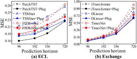
Figure 4 illustrates the performance of applying SoP to each of the three models with prediction horizons S = {96, 192, 336, 720} on the ECL and Exchange datasets. The experimental results demonstrate that the SoP strategy consistently decreases the MSE at diverse prediction horizons. As the prediction horizon expands, the performance improvement brought by SoP becomes increasingly evident, manifested by the growing difference between the solid and dashed lines of the same color.
4.3 Effectiveness of Target-wise SoP (address RQ2)
To investigate the effectiveness of target-wise SoP, we examine the performance SoP with different plug counts on the Weather dataset, which contains a total of 21 target variables.
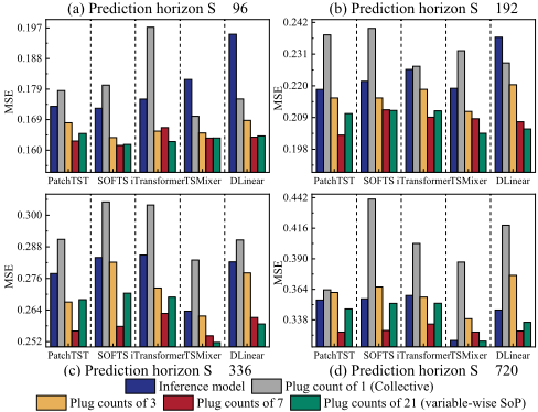
Effect of SoP from Variable View. Given a total of 21 target variables, we specifically setup the plug counts along the Ndimension to form {21, 7, 3, 1} plugs in turn. The experimental results, shown in Figure 5, reveal several key observations. First, most non-collective SoP clearly enhances the performance of inference models, with SoP using plug count of 7 achieving the best performance, followed closely by variablewise SoP. The variable-wise SoP, by eliminating the need to fine-tune the plug count, is thus suggested as a quick-start version of SoP. Second, plug count of 1 (i.e., collective calibrating) generally results in the worst performance, even performing worse than the inference model without calibrating. This suggests the MTLC indeed degrades the performance of most models. Lastly, models with simpler architectures, such as DLinear, benefit more from incorporating SoP.
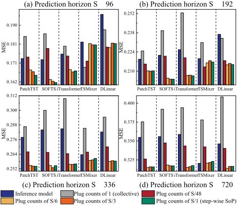
Effect of SoP from Step View. Given that S ∈ {96, 192, 336, 720}, we set up the plug counts along the Sdimension as follows: for S = 96, the plug counts form {96, 32, 16, 2, 1}; for S = 192 , the plug counts form {192, 64, 32, 4, 1}; for S = 336, the plug counts form {336, 128, 64, 8, 1}; and for S = 720, the plug counts form {720, 240, 120, 15, 1}. As shown in Figure 6, the experimental results reveal that MTLC degrades the performance of most models, except for TSMixer, which performs best with collective calibration when S = 96. In contrast, noncollective SoP significantly enhances model performance, with PatchTST, implementing step-wise SoP, achieving the best results across most prediction horizons. Overall, the step-wise SoP, by eliminating the need to experiment with specific plug counts, performs considerably well and can be chosen as a quick-start version of SoP from the step view.
| Model of Socket | SOFTS | iTransformer | DLinear | PatchTST | TimesNet | TSMixer | FEDformer | ||||||||
|---|---|---|---|---|---|---|---|---|---|---|---|---|---|---|---|
| Metric | MSE | MAE | MSE | MAE | MSE | MAE | MSE | MAE | MSE | MAE | MSE | MAE | MSE | MAE | |
| Promotion1 ECL Promotion2 | 2.77% 1.92% | 0.57% 0.05% | 3.41% 3.28% | 0.90% 0.40% | 14.40% 12.72% | 6.96% 6.20% | 9.85% 9.27% | 5.79% 5.54% | 2.68% 3.23% | 1.81% 1.22% | 16.29% 15.59% | 9.80% 9.40% | 9.73% 9.52% | 5.69% 5.55% | |
| Promotion1 Weather Promotion2 | 3.73% 2.72% | 2.49% 1.41% | 4.80% 4.20% | 2.60% 2.04% | 8.97% 5.84% | 6.78% 5.11% | 3.30% 2.49% | 1.84% 1.23% | 0.02% -0.14% | 0.42% -0.06% | 4.69% 3.59% | 3.47% 2.41% | 3.82% 4.56% | 3.27% 5.69% | |
| Promotion1 Exchange Promotion2 | 11.53% 7.03% | -0.82% -0.89% | 22.91% 21.99% | 4.18% 6.10% | 14.68% 4.49% | 3.57% -3.40% | 21.64% 18.60% | 6.78% 3.06% | 19.99% 15.72% | 5.24% 2.86% | 1.37% -5.10% | 1.48% -1.56% | 22.04% 21.22% | 7.49% 7.39% | |
| Traffic Promotion2 | 1.29% | 12.90% | 1.43% 0.91% | 1.11% | 14.13% | 2.07% 0.71% | 1.08% -1.27% | 4.98% | 0.21% | 1.85% | 3.24% | 2.30% | |||
| Promotion1 Promotion1 | 0.56% | 12.85% | 1.37% | 0.84% 0.38% | 12.33% | 13.78% 15.48% | 3.06% | 3.97% | 0.73% | -0.40% | 1.79% 0.64% | 3.91% | 1.31% 1.14% 8.57% | 2.09% | |
| Solar-Energy Promotion2 | 1.25% | 1.14% 0.31% | 1.22% 5.21% | 0.23% 4.77% | 22.36% 21.62% | 22.72% 22.47% | 2.87% | 0.56% -0.53% | -0.30% -6.06% | 0.02% -0.62% | 6.47% | ||||
| Promotion1 | 1.12% | 14.91% | 11.40% | 2.79% | 2.58% | 0.63% | 8.10% | 6.66% | |||||||
| Avg Promotion2 | 3.16% | 2.46% | 6.40% | 4.26% | 3.32% | 6.88% | |||||||||
| 4.82% | 4.95% | 7.09% | |||||||||||||
| Avg | 2.11% | 2.05% | 1.51% | 1.59% | 10.76% | 9.17% | 3.00% | 1.31% | 1.27% | -0.24% | 3.60% | 2.71% | 4.11% | 4.33% | |
4.4 Ablation Study of Non-collective and Collective Optimizer Deployment (address RQ3)
As highlighted by the MTLC phenomenon in Figure 2, we conducted a more rigorous ablation study to compare the effects of non-collective and collective optimizer deployment.
Table 2 summarizes the performance achieved by deploying two different calibrating strategies. The improvements are calculated relative to the performance of the Socket without calibrating, with the superior improvement in each comparison highlighted in bold. Promotion 1 is achieved through variable-wise SoP, where each plug is optimized independently by a specific optimizer. Promotion 2 is achieved via collective calibrating, where all plugs share a unified optimizer. The results show that while both calibrating approaches yield performance improvements, SoP leads to more substantial gains. The average improvement achieved by Promotion 1 is approximately twice that of Promotion 2. A striking example of this difference can be observed with the TSMixer model on the Exchange dataset, where collective calibrating results in a degradation in model performance, while the corresponding SoP strategy leads to significant improvements.
4.5 Experiments on Spatio-temporal Forecasting (address RQ4)
Both time series forecasting and spatio-temporal forecasting aim to predict future values based on historical data, but spatio-temporal forecasting is more complex in terms of data scale and model complexity. This section demonstrates the effectiveness of SoP in spatio-temporal forecasting.
Dataset. The experiments were conducted on the ERA5 dataset [Alibaba Group, 2023], which includes five meteorological variables: T2M, U10, V10, MSL and TP.
Inference model. The inference model selected as the Socket is Unet [Ronneberger et al., 2015]. A direct prediction strategy is employed, which generates predictions for the next 20 prediction horizons without iterative steps.
Experimental settings. For spatio-temporal prediction, a data sample is represented as X ∈ RN×H×W×T , with Y ∈ RN×H×W×S as the corresponding output. In this forecasting task, observations from the past two time steps (T = 2) involving five variables (N = 5) are used to predict the same five variables over the next 20 prediction horizons (S = 20). H ×W denotes the spatial range, with W = H = 160. Experimental results. Next, we provide the analysis of the experimental results in detail.
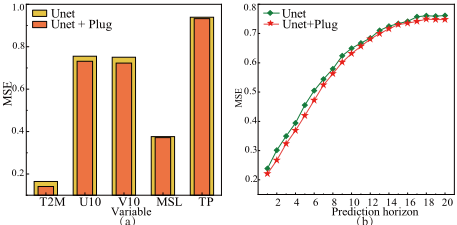
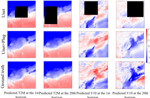
The Effect of SoP on Spatio-temporal Variables. As shown in Figure 7 (a), the averaged test MSE of the five variables significantly decreased after applying SoP to Unet, particularly for the variables T2M, U10, and V10. This improvement can be attributed to the inherently stronger cyclicity of T2M, which enhances its predictability compared to TP and MSL, which aligns with findings in previous studies [Liu et al., 2021]. Figure 8 displays a test sample to visualize the benefits of applying SoP to the Unet model for spatio-temporal predictions of T2M and V10. It can be observed that predictions from Unet alone appear overly smoothed and obscurer at certain spatial locations (highlighted in the black box). In contrast, Unet+SoP produces more textured and sharper predictions that are closer to the ground truth, not only at the first prediction horizon but also at the 20th prediction horizon.
The Effect of SoP on Prediction Horizons. As present in Figure 7 (b), the incorporation of the SoP consistently reduces the test MSE across each of the 20 prediction horizons. Notably, the difference in MSE between Unet+Plug and Unet gradually decreases as the prediction horizon increase. This phenomenon can be attributed to the reduced predictability of spatio-temporal forecasts as the horizon progresses [Bi et al., 2023]. Overall, SoP demonstrates its effectiveness both in short- and long-term spatio-temporal forecasting.
(a)
(b)
Figure 7: (a) The averaged MSE for each of five variables. (b) The averaged MSE at each prediction horizon.
5 RelatedWorks
Forecasting Models. Deep learning has significantly advanced time series forecasting, resulting in the development of numerous deep forecasting models [Deng et al., 2024b]. The architecture of deep models has progressed from CNNsbased frameworks [Wu et al., 2023], MLPs [Zeng et al., 2023] to Transformer [Liu et al., 2024b], achieving considerable performance improvements across various benchmarks. Recently, the rise of LLMs has opened new possibilities for time series forecasting [Liu et al., 2024a; Zhong et al., 2025]. However, some studies have shown that these popular LLMs often perform similarly to, or even worse than, simpler methods, while also significantly increasing computational costs horizon.
horizon.
horizon.
horizon.
Figure 8: Visualization of a spatio-temporal forecasting case study for prediction horizons S=1 and S=20.
during both training and inference [Tan et al., 2024]. As a result, there is no universally superior model architecture in the research community of time series forecasting.
Forecasting Strategies. Recent studies have shown that well-designed forecasting strategies-such as multi-view learning [Deng et al., 2022; Lu et al., 2019] and model calibration-can significantly influence predictive performance. Calibration, in particular, plays a critical role in aligning model predictions with the ground truth [Zhang et al., 2023], or in providing more reliable confidence intervals [Sun et al., 2023]. Early research employed Platt Scaling to transform the original predictions into calibrated probabilities [Platt and others, 1999]. More recently, non-parametric isotonic regression was introduced by [Berta et al., 2024] to calibrate binary classifiers. [Huang et al., 2023] designed an abductive reasoning mechanism to minimize the discrepancy between the inferred and the true values to adjust the predictions. [Zhang et al., 2023] employed the envelope-based bounds modeling to correct the initial predictions. While many previous studies have applied learning-based methods to calibrate model outputs, most have focused on collective calibrating. None of these approaches have noticed the detriment of MTLC in deep forecasting and proposed a solution through noncollective calibrating. To this end, this study has developed an effective calibrating strategy from two views that enhances the performance of deep forecasting models.
6 Conclusions
This study identifies a detrimental phenomenon, termed MTLC, which hampers the learning capability during the training of deep forecasting models. To address this issue, we propose an effective SoP strategy that calibrates well-trained forecasting models, regardless of their specific architectures. Additionally, we derive two specific forms of target-wise SoP for quick-start implementation. Comprehensive experiments demonstrate the superiority of the proposed method, even without exhaustive hyperparameter searching. We hope this approach paves the way for further advancements in time series forecasting. Future research could focus on improving calibrating efficiency through parallel Plug training.
Acknowledgments
This work was supported by the National Natural Science Foundation of China (Nos. 62402463, 41976185, 62176243, 62176221 and 72242106) and Major Basic Research Project of Shandong Provincial Natural Science Foundation (ZR2024ZD03).
Contribution Statement
Bin Wang and Yongqi Han are co-first authors with equal contributions.
@inproceedings{ijcai2025p371,
  title     = {Non-collective Calibrating Strategy for Time Series Forecasting},
  author    = {Wang, Bin and Han, Yongqi and Ma, Minbo and Li, Tianrui and Zhang, Junbo and Hong, Feng and Yu, Yanwei},
  booktitle = {Proceedings of the Thirty-Fourth International Joint Conference on
               Artificial Intelligence, {IJCAI-25}},
  publisher = {International Joint Conferences on Artificial Intelligence Organization},
  editor    = {James Kwok},
  pages     = {3335--3343},
  year      = {2025},
  month     = {8},
  note      = {Main Track},
  doi       = {10.24963/ijcai.2025/371},
  url       = {https://doi.org/10.24963/ijcai.2025/371},
}
TY - CPAPER TI - Non-collective Calibrating Strategy for Time Series Forecasting AU - Wang, Bin AU - Han, Yongqi AU - Ma, Minbo AU - Li, Tianrui AU - Zhang, Junbo AU - Hong, Feng AU - Yu, Yanwei T2 - Proceedings of the Thirty-Fourth International Joint Conference on Artificial Intelligence, IJCAI-25 PB - International Joint Conferences on Artificial Intelligence Organization PY - 2025 SP - 3335 EP - 3343 DO - 10.24963/ijcai.2025/371 UR - https://doi.org/10.24963/ijcai.2025/371 ER -Copied
Machine-readable versions of this paper, for tools and AI agents:





