
Distribution-Aware Online Learning for Urban Spatiotemporal Forecasting on Streaming Data
Proceedings of the Thirty-Fourth International Joint Conference on Artificial Intelligence. Main Track. Pages 3344-3352.
https://doi.org/10.24963/ijcai.2025/372
Keywords
- Data Mining: DM: Mining spatial and/or temporal data
- Data Mining: DM: Mining data streams
Abstract
The intrinsic non-stationarity of urban spatiotemporal (ST) streams, particularly unique distribution shifts that evolve over time, poses substantial challenges for accurate urban ST forecasting. Existing works often overlook these dynamic shifts, limiting their ability to adapt to evolving trends effectively. To address this challenge, we propose DOL, a novel Distribution-aware Online Learning framework designed to handle the unique shifts in urban ST streams. DOL introduces a streaming update mechanism that leverages streaming memories to strategically adapt to gradual distribution shifts. By aligning network updates with these shifts, DOL avoids unnecessary updates, reducing computational overhead while improving prediction accuracy. DOL also incorporates an adaptive spatiotemporal network with a location-specific learner, enabling it to handle diverse urban distribution shifts across locations. Experimental results on four real-world datasets confirm DOL's superiority over state-of-the-art models. The source code is available at https://github.com/cwang-nus/DOL.
- [Bai et al., 2020] Lei Bai, Lina Yao, Can Li, Xianzhi Wang, and Can Wang. Adaptive graph convolutional recurrent network for traffic forecasting. NeurIPS, 33, 2020.
- [Brockwell et al., 2016] Peter J Brockwell, Peter J Brock- well, Richard A Davis, and Richard A Davis. Introduction to time series and forecasting. Springer, 2016.
- [Buzzega et al., 2020] Pietro Buzzega, Matteo Boschini, An- gelo Porrello, Davide Abati, and Simone Calderara. Dark experience for general continual learning: a strong, simple baseline. NeurIPS, 33:15920-15930, 2020.
- [Cermelli et al., 2022] Fabio Cermelli, Dario Fontanel, An- tonio Tavera, Marco Ciccone, and Barbara Caputo. In- cremental learning in semantic segmentation from image labels. In CVPR, pages 4371-4381, 2022.
- [Chaudhry et al., 2019] Arslan Chaudhry, Marcus Rohrbach, Mohamed Elhoseiny, Thalaiyasingam Ajanthan, Puneet K Dokania, Philip HS Torr, and Marc'Aurelio Ranzato. On tiny episodic memories in continual learning. arXiv, 2019.
- [Chen et al., 2021] Xu Chen, Junshan Wang, and Kunqing Xie. Trafficstream: A streaming traffic flow forecasting framework based on graph neural networks and continual learning. In IJCAI, 2021. IJCAI
- [Cruz and Sarmento, 2021] Carlos Oliveira Cruz and Joaquim Miranda Sarmento. The impact of covid-19 on highway traffic and management: The case study of an operator perspective. Sustainability, 2021.
- [Deng et al., 2021] Jinliang Deng, Xiusi Chen, Renhe Jiang, Xuan Song, and Ivor W Tsang. St-norm: Spatial and tem- poral normalization for multi-variate time series forecast- ing. In SIGKDD, 2021.
- [Douillard et al., 2021] Arthur Douillard, Yifu Chen, Ar- naud Dapogny, and Matthieu Cord. Plop: Learning with- out forgetting for continual semantic segmentation. In CVPR, pages 4040-4050, 2021.
- [Gao and Glowacka, 2016] Yuan Gao and Dorota Glowacka. Deep gate recurrent neural network. In Asian conference on machine learning, pages 350-365. PMLR, 2016.
- [Gunasekara et al., 2023] Nuwan Gunasekara, Bernhard Pfahringer, Heitor Murilo Gomes, and Albert Bifet. Survey on online streaming continual learning. In IJCAI, pages 6628-6637, 2023. IJCAI
- [Han et al., 2024] Jindong Han, Weijia Zhang, Hao Liu, Tao Tao, Naiqiang Tan, and Hui Xiong. Bigst: Linear com- plexity spatio-temporal graph neural network for traffic forecasting on large-scale road networks. VLDB, 2024.
- [Harun et al., 2023] Md Yousuf Harun, Jhair Gallardo, Tyler L. Hayes, Ronald Kemker, and Christopher Kanan. SIESTA: efficient online continual learning with sleep. Trans. Mach. Learn. Res., 2023.
- [Hochreiter and Schmidhuber, 1997] Sepp Hochreiter and Jürgen Schmidhuber. Long short-term memory. Neural computation, 1997. [Houlsby et al., 2019] Neil Houlsby, Andrei Giurgiu, Stanis- law Jastrzebski, Bruna Morrone, Quentin De Laroussilhe, Andrea Gesmundo, Mona Attariyan, and Sylvain Gelly. Parameter-efficient transfer learning for nlp. In ICML, pages 2790-2799, 2019.
- [Hu et al., 2022] Edward J. Hu, Yelong Shen, Phillip Wallis, Zeyuan Allen-Zhu, Yuanzhi Li, Shean Wang, Lu Wang, and Weizhu Chen. Lora: Low-rank adaptation of large language models. In ICLR, 2022.
- [Jiang et al., 2023] Jiawei Jiang, Chengkai Han, Wayne Xin Zhao, and Jingyuan Wang. Pdformer: Propagation delay- aware dynamic long-range transformer for traffic flow pre- diction. In AAAI, 2023.
- [Kim et al., 2021] Taesung Kim, Jinhee Kim, Yunwon Tae, Cheonbok Park, Jang-Ho Choi, and Jaegul Choo. Re- versible instance normalization for accurate time-series forecasting against distribution shift. In ICLR, 2021.
- [Lee and Ko, 2024] Hyunwook Lee and Sungahn Ko. TES- TAM: A time-enhanced spatio-temporal attention model with mixture of experts. In ICLR, 2024.
- [Li et al., 2018a] Yaguang Li, Kun Fu, Zheng Wang, Cyrus Shahabi, Jieping Ye, and Yan Liu. Multi-task representa- tion learning for travel time estimation. In SIGKDD, 2018.
- [Li et al., 2018b] Yaguang Li, Rose Yu, Cyrus Shahabi, and Yan Liu. Diffusion convolutional recurrent neural net- work: Data-driven traffic forecasting. In ICLR, 2018.
- [Liu et al., 2022] Dachuan Liu, Jin Wang, Shuo Shang, and Peng Han. Msdr: Multi-step dependency relation networks for spatial temporal forecasting. In SIGKDD, 2022.
- [Liu et al., 2023] Hangchen Liu, Zheng Dong, Renhe Jiang, Jiewen Deng, Jinliang Deng, Quanjun Chen, and Xuan Song. Spatio-temporal adaptive embedding makes vanilla transformer sota for traffic forecasting. In CIKM, 2023.
- [Lopez-Paz and Ranzato, 2017] David Lopez-Paz and Marc'Aurelio Ranzato. Gradient episodic memory for continual learning. NeurIPS, 30, 2017.
- [Lu et al., 2018] Jie Lu, Anjin Liu, Fan Dong, Feng Gu, Joao Gama, and Guangquan Zhang. Learning under concept drift: A review. TKDE, 31(12), 2018.
- [Miao et al., 2024] Hao Miao, Yan Zhao, Chenjuan Guo, Bin Yang, Kai Zheng, Feiteng Huang, Jiandong Xie, and Christian S Jensen. A unified replay-based continu- ous learning framework for spatio-temporal prediction on streaming data. ICDE, 2024.
- [Nie et al., 2023] Yuqi Nie, Nam H. Nguyen, Phanwadee Sinthong, and Jayant Kalagnanam. A time series is worth 64 words: Long-term forecasting with transformers. In ICLR, 2023.
- [Pfeiffer et al., 2020] Jonas Pfeiffer, Ivan Vulic, Iryna Gurevych, and Sebastian Ruder. MAD-X: an adapter- based framework for multi-task cross-lingual transfer. In EMNLP, pages 7654-7673, 2020.
- [Pham et al., 2023] Quang Pham, Chenghao Liu, Doyen Sa- hoo, and Steven C. H. Hoi. Learning fast and slow for online time series forecasting. In ICLR, 2023.
- [Qian and Ukkusuri, 2015] Xinwu Qian and Satish V Ukkusuri. Spatial variation of the urban taxi ridership using gps data. Applied geography, 59:31-42, 2015.
- [Shao et al., 2022] Zezhi Shao, Zhao Zhang, Fei Wang, Wei Wei, and Yongjun Xu. Spatial-temporal identity: A simple yet effective baseline for multivariate time series forecast- ing. In CIKM, pages 4454-4458, 2022.
- [Shao et al., 2025] Zezhi Shao, Fei Wang, Yongjun Xu, Wei Wei, Chengqing Yu, Zhao Zhang, Di Yao, Guangyin Jin, Xin Cao, Gao Cong, et al. Exploring progress in mul- tivariate time series forecasting: Comprehensive bench- marking and heterogeneity analysis. IEEE Trans. Knowl. Data Eng., 2025.
- [Shi and Li, 2018] Hongzhi Shi and Yong Li. Discover- ing periodic patterns for large scale mobile traffic data: Method and applications. IEEE TMC, 17(10), 2018.
- [Vaswani et al., 2017] Ashish Vaswani, Noam Shazeer, Niki Parmar, Jakob Uszkoreit, Llion Jones, Aidan N Gomez, Łukasz Kaiser, and Illia Polosukhin. Attention is all you need. NeurIPS, 2017.
- [Vitter, 1985] Jeffrey S Vitter. Random sampling with a reservoir. TOMS, 11(1):37-57, 1985.
- [Wang et al., 2022] Chengxin Wang, Yuxuan Liang, and Gary Tan. Periodic residual learning for crowd flow fore- casting. In SIGSPATIAL, pages 1-10, 2022.
- [Wang et al., 2023a] Binwu Wang, Yudong Zhang, Xu Wang, Pengkun Wang, Zhengyang Zhou, Lei Bai, and Yang Wang. Pattern expansion and consolidation on evolving graphs for continual traffic prediction. In SIGKDD, pages 2223-2232, 2023.
- [Wang et al., 2023b] Kuo Wang, LingBo Liu, Yang Liu, GuanBin Li, Fan Zhou, and Liang Lin. Urban regional function guided traffic flow prediction. Information Sci- ences, 634:308-320, 2023.
- [Wang et al., 2024] Chengxin Wang, Yuxuan Liang, and Gary Tan. Citycan: Causal attention network for citywide spatio-temporal forecasting. In WSDM, 2024.
- [Wang et al., 2025] Chengxin Wang, Yiran Zhao, Shaofeng Cai, and Gary Tan. Investigating pattern neurons in urban time series forecasting. In ICLR, 2025.
- [Wen et al., 2024] Qingsong Wen, Weiqi Chen, Liang Sun, Zhang Zhang, Liang Wang, Rong Jin, Tieniu Tan, et al. Onenet: Enhancing time series forecasting models under concept drift by online ensembling. NeurIPS, 36, 2024.
- [Williams and Hoel, 2003] Billy M Williams and Lester A Hoel. Modeling and forecasting vehicular traffic flow as a seasonal arima process: Theoretical basis and empirical results. J. Transp. Eng., 129(6):664-672, 2003.
- [Wu et al., 2019] Zonghan Wu, Shirui Pan, Guodong Long, Jing Jiang, and Chengqi Zhang. Graph wavenet for deep spatial-temporal graph modeling. In IJCAI, 2019. IJCAI
- [Wu et al., 2020] Zonghan Wu, Shirui Pan, Guodong Long, Jing Jiang, Xiaojun Chang, and Chengqi Zhang. Con- necting the dots: Multivariate time series forecasting with graph neural networks. In SIGKDD, pages 753-763, 2020.
- [Xia et al., 2023] Yutong Xia, Yuxuan Liang, Haomin Wen, Xu Liu, Kun Wang, Zhengyang Zhou, and Roger Zimmer- mann. Deciphering spatio-temporal graph forecasting: A causal lens and treatment. NeurIPS, 2023.
- [Yao et al., 2018] Huaxiu Yao, Fei Wu, Jintao Ke, Xianfeng Tang, Yitian Jia, Siyu Lu, Pinghua Gong, Jieping Ye, and Zhenhui Li. Deep multi-view spatial-temporal network for taxi demand prediction. In AAAI, volume 32, 2018.
- [Yu and Peng, 2019] Haitao Yu and Zhong-Ren Peng. Ex- ploring the spatial variation of ridesourcing demand and its relationship to built environment and socioeconomic fac- tors with the geographically weighted poisson regression. Journal of Transport Geography, 75:147-163, 2019.
- [Yu et al., 2018] Bing Yu, Haoteng Yin, and Zhanxing Zhu. Spatio-temporal graph convolutional networks: A deep learning framework for traffic forecasting. In IJCAI, 2018. IJCAI
- [Zeng et al., 2023] Ailing Zeng, Muxi Chen, Lei Zhang, and Qiang Xu. Are transformers effective for time series fore- casting? In AAAI, volume 327, pages 11121-11128, 2023.
- [Zhang et al., 2017] Junbo Zhang, Yu Zheng, and Dekang Qi. Deep spatio-temporal residual networks for citywide crowd flows prediction. In AAAI, 2017.
- [Zhang et al., 2021] Xiyue Zhang, Chao Huang, Yong Xu, Lianghao Xia, Peng Dai, Liefeng Bo, Junbo Zhang, and Yu Zheng. Traffic flow forecasting with spatial-temporal graph diffusion network. In AAAI, 2021.
- [Zhang et al., 2024] Renrui Zhang, Jiaming Han, Chris Liu, Aojun Zhou, Pan Lu, Yu Qiao, Hongsheng Li, and Peng Gao. Llama-adapter: Efficient fine-tuning of large lan- guage models with zero-initialized attention. In ICLR, 2024.
- [Zhao et al., 2023] Wei Zhao, Shiqi Zhang, Bei Wang, and Bing Zhou. Spatio-temporal causal graph attention net- work for traffic flow prediction in intelligent transportation systems. PeerJ Computer Science, 9, 2023.
- [Zheng et al., 2020] Chuanpan Zheng, Xiaoliang Fan, Cheng Wang, and Jianzhong Qi. Gman: A graph multi-attention network for traffic prediction. In AAAI, volume 34, pages 1234-1241, 2020.
- [Zhou et al., 2023a] Tian Zhou, Peisong Niu, Xue Wang, Liang Sun, and Rong Jin. One fits all: Power general time series analysis by pretrained LM. In NeurIPS, 2023.
- [Zhou et al., 2023b] Zhengyang Zhou, Qihe Huang, Kuo Yang, Kun Wang, Xu Wang, Yudong Zhang, Yuxuan Liang, and Yang Wang. Maintaining the status quo: Cap- turing invariant relations for ood spatiotemporal learning. SIGKDD, 2023.
- [Zhou et al., 2024] Yicheng Zhou, Pengfei Wang, Hao Dong, Denghui Zhang, Dingqi Yang, Yanjie Fu, and Pengyang Wang. Make graph neural networks great again: A generic integration paradigm of topology-free patterns for traffic speed prediction. In IJCAI, 2024. IJCAI
- [Zinkevich, 2003] Martin Zinkevich. Online convex pro- gramming and generalized infinitesimal gradient ascent. In ICML, 2003.
References were extracted automatically from the PDF and may contain errors.
Full text extracted automatically from the PDF; figures, tables and equations may differ. The PDF is the version of record.
1 Introduction
Urban spatiotemporal (ST) forecasting is a crucial task in Intelligent Transportation Systems (ITS), enabling various smart city solutions such as intelligent scheduling [Yao et al., 2018; Lee and Ko, 2024], effective traffic management [Zhang et al., 2021; Wang et al., 2023b], and optimal trip planning [Li et al., 2018a; Han et al., 2024]. While recent advances in ST forecasting models [Wu et al., 2019; Liu et al., 2022] have greatly improved accuracy, their effectiveness in urban ST streams is hindered by the oversight of intrinsic distribution shifts arising from continuous data flow.
While distribution shifts in urban ST streams occur over time, they evolve gradually because of the stable nature of urban zoning and functionality [Qian and Ukkusuri, 2015; Yu and Peng, 2019]. As illustrated in Figure 1, taxi demand in Chicago exhibits significant variations over months (e.g., January to March) but remains stable over shorter intervals, such as consecutive weeks (see substantially similar distributions marked in red and yellow). However, most urban ST forecasting methods [Wu et al., 2019; Jiang et al., 2023; Lee and Ko, 2024] are conducted with static training samples and neglect such distribution shifts. Recent efforts to address these shifts fall into offline and online adaptation models. Offline models rely on historical data to alleviate discrepancies through learnable normalization [Kim et al., 2021; Nie et al., 2023] or enable generalization with invariant correlations [Xia et al., 2023; Zhou et al., 2023b], but struggle with shifts during unforeseen events like COVID-19 [Cruz and Sarmento, 2021]. Online adaptation models address this issue by leveraging incoming data with batch updates, which update the network annually [Chen et al., 2021; Wang et al., 2023a; Miao et al., 2024], or immediate updates, which fine-tune the network as new data arrives [Pham et al., 2023; Wen et al., 2024]. However, batch updates are insufficient for intra-year shifts, while immediate updates are computationally expensive and risk overfitting due to frequent updates.
∗ Work was partially done when the author interned at Comfort Transportation Pte Ltd.
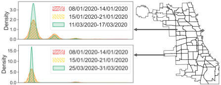
Beyond gradual distribution shifts, different urban locations also exhibit unique patterns shaped by location-specific factors such as urban functionality [Yu and Peng, 2019]. As illustrated in Figure 1, the estimated data distributions in Region 23 (residential area) and Region 64 (transportation hub) differ significantly and vary considerably over extended periods (e.g., January to March 2020; see distributions marked in yellow and green). Such shifts make prior adaptation strategies [Chaudhry et al., 2019; Pham et al., 2023] ineffective for existing ST forecasting models, which lack mechanisms for location-specific learning. Moreover, these strategies often require full network fine-tuning, which is computationally expensive. Recent proposals, such as parameter-efficient tuning [Houlsby et al., 2019; Hu et al., 2022], selectively fine-tune specific components, providing a more efficient approach to network adaptation. However, they still fail to handle the unique shifts at individual locations.
In this paper, we propose DOL, a distribution-aware online learning framework that leverages the unique distributions of urban ST streams for accurate forecasting. DOL provides a novel online adaptation strategy aligned with the nature of urban ST streams: it alternates the network update between awake and hibernate phases, allowing the network to mitigate performance degradation caused by evolving distribution shifts while reducing unnecessary updates and computational costs for gradual shifts. To facilitate effective forecasting on incoming streams, it employs a Streaming Update Mechanism (SUM) that fine-tunes specific network parameters using an episodic memory of relevant samples, ensuring efficient adaptation and preventing both overfitting and catastrophic forgetting. In addition, we introduce an adaptive ST network, AST-Net, equipped with a plug-and-play component named the Location-Specific Learner (LSL). LSL precisely learns new distribution patterns for each urban location over time, customizing learners to effectively fine-tune the network in response to location-specific distribution shifts.
Our main contributions are summarized as follows:
- We propose DOL, a novel distribution-aware online learning framework tailored for urban ST forecasting that finetunes the network to align with gradual urban distribution shifts over time, thus enabling network adaptation while avoiding inefficient training.
- We introduce the Location-Specific Learner LSL, which enables the network to adapt to diverse and evolving urban distribution shifts across different locations.
- Extensive experimental results confirm DOL's superiority over state-of-the-art methods on four real-world datasets, reducing forecast errors by 12.89% over 13 baselines.
2 RelatedWork
Urban Spatiotemporal (ST) Forecasting is a critical task in smart city development, which supports various urban applications. Early methods relied on statistical models, such as HA [Brockwell et al., 2016], ARIMA [Williams and Hoel, 2003], etc. Recent advances utilize deep models to capture ST correlations and thus significantly improve forecasting. They typically employ graph neural networks [Wu et al., 2019; Zheng et al., 2020] or attentions [Zhao et al., 2023; Zhou et al., 2024; Wang et al., 2025] for dynamic spatial modeling; RNNs [Hochreiter and Schmidhuber, 1997; Gao and Glowacka, 2016], CNNs [Zhang et al., 2017; Wang et al., 2022], or Transformers [Vaswani et al., 2017; Liu et al., 2023] for temporal modeling; and normalization [Deng et al., 2021] or identity embedding [Shao et al., 2022; Liu et al., 2023] for ST feature learning. However, these approaches often overlook temporal dynamics during test time. Some studies address this out-of-distribution issue in offline settings by applying learnable normalization [Kim et al., 2021; Nie et al., 2023] or identifying invariant relationships [Zhou et al., 2023b; Wang et al., 2024]. Nonetheless, they still struggle with online streams, where invariant relationships evolve over time, particularly during unforeseen events [Cruz and Sarmento, 2021]. While some works adopt continual learning to handle such shifts [Chen et al., 2021; Miao et al., 2024], they divide the stream into tasks and delay updates until substantial data accumulates, resulting in infrequent updates that limit their timely adaptation.
Online Learning focuses on adapting to shifts in data distribution and has proven highly effective in various tasks, from image classification [Buzzega et al., 2020; Harun et al., 2023; Gunasekara et al., 2023] to natural language processing [Houlsby et al., 2019; Pfeiffer et al., 2020]. Recent research has extended online learning to time series models to address distribution shifts in data streams. For instance, FSNet [Pham et al., 2023] utilizes memory mechanisms for data adaptation, while OneNet [Wen et al., 2024] employs reinforcement learning to adjust weights between two forecasters during the online phase. However, these models are designed for unstable temporal patterns [Shao et al., 2025] and employ full fine-tuning, which is unnecessary for gradual distribution shifts and introduce high computation overhead. Recently, adapter-based frameworks [Houlsby et al., 2019; Zhou et al., 2023a; Zhang et al., 2024] have demonstrated remarkable effectiveness and efficiency in handling unseen tasks by fine-tuning selective network layers. Meanwhile, SIESTA [Harun et al., 2023] demonstrates that a sleep mechanism can achieve efficient online image classification. Nevertheless, these models lack effective ST modeling and thus cannot be directly applied to urban ST forecasting.
3 Preliminaries
Definition 1 (Urban Spatiotemporal Data). In the urban context, 𝑁 spatially distributed sensors (e.g., traffic sensors) form a spatial graph G based on their geographical locations. At each time 𝜏, urban conditions (e.g., taxi demand, traffic speed) are represented as 𝑋𝜏 ∈ R 𝑁×𝑑 , where 𝑑 is the feature dimension. Urban spatiotemporal (ST) data over the interval [𝜏, 𝜏 +𝑇] is denoted as 𝑋𝜏:𝜏+𝑇 ∈ R 𝑁×(𝑇+1)×𝑑 .
Definition 2 (External Factors). External factors such as time of day and day of the week influence urban ST data by reflecting daily routines and weekly cycles [Zhang et al., 2017]. We denote the external factors at time 𝜏 as 𝐸𝜏.
Online Urban STForecasting. In urban scenarios, data arrives as a stream, denoted as 𝑋𝜏:∞. The goal is to process this stream and forecast traffic conditions across urban locations for the next 𝐻 time steps at each time 𝜏, given external factors 𝐸 and past observations from a look-back window 𝐿:
where 𝑓 (·) represents the learnable ST network. For simplicity, we denote the 𝐿 observations as X𝜏 and the 𝐻 predictions as Y𝜏 in the following sections.
4 Methodology
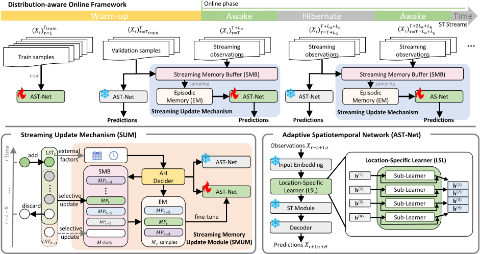
In this section, we introduce DOL for urban ST forecasting, as depicted in Figure 2. DOL comprises two key components: the Streaming Update Mechanism (SUM), which manages network fine-tuning to address gradual distribution shifts, and the Adaptive ST Network (AST-Net), which enables the network to adapt to location-specific shifts. To process online ST streams, DOL consists of Warm-up and Online phases. Algorithm 1 outlines DOL for online urban ST forecasting.
4.1 Phases for Online ST Forecasting
Conventional ST networks, trained on static datasets, often struggle to adapt to distribution shifts over extended inference periods. To address this, DOL leverages online learning, enabling its ST network AST-Net, to adapt to newly emerging patterns during the Online phase (i.e., test time in an offline setting). The phases for DOL consist of a Warm-up phase for initial training and an Online phase for fine-tuning with evolving patterns. Moreover, to accommodate gradual distribution shifts, DOL intermittently pauses fine-tuning during the Online phase to prevent excessive updates.
Warm-up Phase. Warm-up Phase prepares the network for online ST forecasting. During this phase, the AST-Net of DOL is trained and validated, similar to offline ST networks [Wu et al., 2019; Jiang et al., 2023], before performing the forecasting task. To mitigate potential distribution shifts during validation, DOL selectively stores relevant samples in a Streaming Memory Buffer (SMB) to support fine-tuning at the beginning of the Online phase (details in Section 4.2).
Online Phase. Online Phase performs forecasting with AST-Net at each time step. During this phase, DOL intermittently fine-tunes AST-Net to adapt to gradual distribution shifts, thus forming Awake and Hibernate phases. During Awake phases, the network adapts to distribution shifts, while during Hibernate phases, updates are paused to align with the nature of urban ST streams. This strategy leverages the stable nature of data distributions over short periods, where the discrepancy between consecutive short periods is negligible:
where 𝑃(D1) and 𝑃(D2) denote the data distributions for consecutive short periods D1 and D2. Thus, the network finetuned on D1 can generalize to D2 without further updates.
The transition between the Awake and Hibernate phases, along with network updates in the Awake phase, is managed by SUM (details in Section 4.2). During the Awake phase, the Streaming Memory Buffer (SMB) within SUM is updated with newly arriving samples, and the AST-Net is fine-tuned to adapt to evolving patterns using the updated SMB. Conversely, during the Hibernate phase, only the SMB is updated, while network fine-tuning is paused to conserve computational resources, as short-term shifts remain stable.
4.2 Streaming Update Mechanism
The Streaming Update Mechanism (SUM), shown in Figure 2 (lower-left), manages phase transitions and fine-tunes the network during the Awake phase. It comprises two components: the Latest Sample Tracker (LST) and the Streaming Memory
Algorithm 1: Online urban ST forecasting
Input: Network 𝑓 (·) learned during the warm-up phase, including parameters 𝜃𝑡 for traditional modules and 𝜃𝑎 for the adapter; Validation dataset D𝑣𝑎𝑙 ; The length of the look-back window 𝐿 and prediction horizon 𝐻; The length of the awake and AH periods 𝐿𝑎 and 𝐿𝑎ℎ; The latest sample tracker 𝐿𝑆𝑇; Online data stream [𝑋𝜏 , 𝑋𝜏+1, · · · , 𝑋∞].
1 M← ∅ ; // Set the SMB to empty 2 𝑎𝑤𝑎𝑘𝑒 ← 𝑡𝑟𝑢𝑒 ; // Awake at the first step // Update the SMB with validation data 3 foreach (X𝑣𝑎𝑙 , Y𝑣𝑎𝑙 ) ∈ D𝑣𝑎𝑙 do 4 M←M∪ { (X𝑣𝑎𝑙 , Y𝑣𝑎𝑙 ) } ; // Update SMB // Online phase 5 foreach 𝜏 ∈ [0, ∞) do 6 𝐿𝑆𝑇𝜏 ← 𝑋𝜏 ; // Update LST 7 if 𝜏 ≥ 𝐻 then 8 𝐿𝑆𝑇 𝑥 𝜏 = 𝑋𝜏-𝐿-𝐻:𝜏-𝐻 9 𝐿𝑆𝑇 𝑦 𝜏 = 𝑋𝜏-𝐻+1:𝜏 10 M ← M ∪ { (𝐿𝑆𝑇 𝑥 𝜏 , 𝐿𝑆𝑇 𝑦 𝜏 ) } ; // Update SMB 11 if 𝑎𝑤𝑎𝑘𝑒 then // Fine-tune the network 12 Sample a small M𝑒 from M; 13 foreach 𝑋𝑒 ∈ M𝑒 do 14 ˆY𝑒 = 𝑓 (X𝑒); 15 𝜃𝑎 ← L( ˆY𝑒 , Y𝑒 ) 16 ˆY𝜏 = ˆX𝜏+1:𝜏+𝐻 = 𝑓 (X𝜏-𝐿:𝜏 ) ; // Forecasts // Decide awake or hibernate for next time step 17 if 𝜏 % 𝐿𝑎 == 0 and 𝑎𝑤𝑎𝑘𝑒 then 18 𝑎𝑤𝑎𝑘𝑒 ← 𝑓 𝑎𝑙𝑠𝑒 19 M← ∅ ; // set SMB to empty 20 else if 𝜏 % 𝐿𝑎ℎ == 0 and 𝑛𝑜𝑡 𝑎𝑤𝑎𝑘𝑒 then 21 𝑎𝑤𝑎𝑘𝑒 ← 𝑡𝑟𝑢𝑒Update Module (SMUM). These components enable SUM to address two key challenges of continuous fine-tuning during the Awake phase: (1) delayed ground truth, where at each time step 𝑋𝜏, the network receives only the current observation 𝑋𝜏, while the ground truth 𝑋𝜏+1:𝜏+𝐻 remains unavailable, making immediate fine-tuning impractical; (2) catastrophic forgetting, where frequent updates cause the network to forget earlier patterns [Lu et al., 2018], such as forgetting Monday's patterns by Sunday during a one-week update.
Latest Sample Tracker
The Latest Sample Tracker (LST) addresses delayed ground truth by tracking the most recent samples. At each time step 𝜏, it maintains the latest observations 𝐿𝑆𝑇𝜏 = 𝑋𝜏-𝐿-𝐻+1:𝜏 ∈ R 𝑁×(𝐿+𝐻)×𝑑 by discarding the oldest data 𝑋𝜏-𝐿-𝐻 and incorporating the new data 𝑋𝜏. Thus, it allows DOL to retain the latest observations without revisiting the entire sequence. The updated 𝐿𝑆𝑇𝜏 is then passed to the SMUM, enabling AST-Net to efficiently adapt to recent trends while eliminating the need for the future sequence 𝑋𝜏+1:𝜏+𝐻.
Streaming Memory Update Module
Recent studies [Chaudhry et al., 2019; Lopez-Paz and Ranzato, 2017] have proven that a tiny memory of previously trained samples can mitigate catastrophic forgetting and thus stabilize training during network updates. Inspired by them, we propose a Streaming Memory Update Module (SMUM) to address catastrophic forgetting for urban ST forecasting. SMUM includes a Streaming Memory Buffer (SMB) to store relevant trained samples, an Awake-Hibernate (AH) Decider to determine the current phase, and an Episodic Memory (EM) to select pertinent samples for network updates.
Streaming Memory Buffer (SMB). Unlike prior works that store all past samples [Chaudhry et al., 2019; Lopez-Paz and Ranzato, 2017], our SMB M is tailored for urban ST streams by selectively retaining only the most relevant samples. Specifically, it prioritizes samples from the most recent Awake-Hibernate (AH) phase because: (1) distant past data can become irrelevant due to evolving patterns, and (2) recurrent patterns often emerge within a single AH cycle due to gradual shifts and weekly periodicity [Wang et al., 2022].
The SMB M has 𝑀 slots to store observations from the LST. At the start of each Hibernate phase, M is reset to ensure it retains only the latest AH cycle data. During the online phase, M is updated at each time step 𝜏 with the current observation 𝐿𝑆𝑇𝜏 using reservoir sampling [Vitter, 1985]. Thus, M at time 𝜏 can be represented as:
where 𝐿𝑆𝑇 𝑥 𝜏 = 𝑋𝜏-𝐿-𝐻+1:𝜏-𝐻 ∈ R 𝑁×𝐿×𝑑 and 𝐿𝑆𝑇 𝑦 𝜏 = 𝑋𝜏-𝐻+1:𝜏 ∈ R 𝑁×𝐻×𝑑 , 𝐿𝑎ℎ is the duration of an AH cycle, and the probability of storing 𝐿𝑆𝑇𝜏 in the SMB is 𝑀/𝐿𝑎ℎ.
Awake-Hibernate (AH) Decider. The AH Decider determines whether a given time step 𝜏 falls into the Awake or Hibernate phase by leveraging external factors, such as date and time, to align the schedule with weekly patterns in urban ST data [Shi and Li, 2018; Wang et al., 2022]. An AH cycle has a total length of 𝐿𝑎ℎ = 𝐿𝑎 + 𝐿ℎ, where 𝐿𝑎 and 𝐿ℎ are the durations of the Awake and Hibernate phases, respectively, and 𝐿ℎ = 𝜆𝐿𝑎 ∝ 𝐿𝑤, with 𝐿𝑤 as the length of a week and 𝜆 as the AH parameter. During the Awake phase, the AST-Net is finetuned before generating forecasts, whereas in the Hibernate phase, it generates forecasts without fine-tuning.
Episodic Memory (EM). Our EM randomly selects a subset M𝑒 from M to update the network during the Awake phase. The selected M𝑒, with size 𝑀𝑒 ≪ 𝑀, includes only data from the most recent AH cycle up to time 𝜏, serving to: (1) incorporate recent patterns to prevent catastrophic forgetting, and (2) introduce randomness to avoid overfitting. Note that M𝑒 may not contain the very latest samples, such as 𝐿𝑆𝑇 𝑥 𝜏 and 𝐿𝑆𝑇 𝑦 𝜏 , as random sampling fromM is employed. However, this is sufficient to capture recent patterns, as distribution shifts within an AH cycle are generally stable.
Optimization. Our SMUM optimizes the network for urban ST streams, differing from prior studies in four key aspects: (1) it updates the network only during Awake phases, instead of immediately upon receiving new data [Douillard et al., 2021; Cermelli et al., 2022]; (2) it selects EM from the most relevant samples to preserve recent knowledge, rather than randomly sampling from all past observations [Chaudhry et al., 2019; Miao et al., 2024], which often misses recent trends; (3) it does not explicitly incorporate the latest sample for network updates, unlike methods that update based on the most recent data [Pham et al., 2023;
Wen et al., 2024]; (4) it fine-tunes only a subset of network parameters to reduce computational costs, instead of finetuning all parameters [Chaudhry et al., 2019; Pham et al., 2023]. The optimization function during the Awake phase is:
where 𝜃𝑎 refers to the learnable parameters fine-tuned during the Awake phase, specifically the parameters in the LocationSpecific Learner (LSL) in practice, 𝑀𝐴𝐸 denotes the Mean Absolute Error, and ˆY𝑒 and Y𝑒 ∈ R 𝑀𝑒×𝑁×𝐻×𝑑 are the predictions and ground truth based on M𝑒, where 𝑑 represents the dimension for the target urban condition. Note that the optimization function for DOL during the Warm-up phase follows prior works [Wu et al., 2019; Jiang et al., 2023]:
where 𝜃 represents the learnable parameters of AST-Net, 𝜃𝑡 denotes the subset of 𝜃 excluding 𝜃𝑎, and ˆY and Y ∈ R 𝑁×𝐻×𝑑 are the predictions and ground truth for the training samples.
4.3 Adaptive Spatiotemporal Network
Distribution shifts during the Online phase can vary widely across urban locations. For example, school areas may experience drastic changes during holidays, while CBD regions remain stable. Prior works [Wu et al., 2019; Wu et al., 2020] have focused on improving ST correlation modeling but lack location-specific learning, limiting their adaptability to such shifts over time. To address this, DOL employs an Adaptive Spatiotemporal Network (AST-Net), as shown in the lower right of Figure 2. Alongside the standard modules of ST networks [Yu et al., 2018; Wu et al., 2019] like Input Embedding (IE), ST Module, and Decoder, AST-Net inserts a LocationSpecific Learner (LSL) between the IE and ST Module to enable precise adaptation to location-specific shifts while preventing interference from irrelevant shifts in other locations.
Location-Specific Learner (LSL). LSL is a plug-and-play component, as shown on the right of AST-Net in Figure 2. It takes input embeddings h ∈ R 𝑁×𝐿×𝑑ℎ from the IE and generates adapted embeddings ˜h ∈ R 𝑁×𝐿×𝑑ℎ . These adapted embeddings are then passed to the ST Module for ST correlations modeling and subsequently to the Decoder to generate future urban ST conditions ˆY. Specifically, LSL comprises 𝑁 sub-learners, each designed to handle distribution shifts for a specific location 𝑛. For each location, the corresponding sublearner transforms the input embedding h (𝑛) ∈ R 𝐿×𝑑ℎ into a location-specific adapted embedding ˜h (𝑛) ∈ R 𝐿×𝑑ℎ . The final output of LSL ˜h ∈ R 𝑁×𝐿×𝑑ℎ is obtained by concatenating the adapted embeddings ˜h (𝑛) across all 𝑁 locations:
where 𝑓𝑎 is a non-linear transformation function (e.g., a multi-layer perceptron), 𝜎 is the ReLU activation, W (𝑛) 𝑎 are the learnable parameters for location 𝑛, with W (𝑛) 𝑎1 ∈ R 𝑑ℎ×𝑑𝑚 and W (𝑛) 𝑎2 ∈ R 𝑑𝑚×𝑑ℎ ; 𝑑ℎ is the input feature dimension, concat denotes concatenation along the location dimension, and 𝑑𝑚 ≪ 𝑑ℎ ensures manageable parameter usage.
By default, we adopt the IE, ST Module, and Decoder from GWNet [Wu et al., 2019]. LSL is placed before the ST Module because the latter aggregates both spatial and temporal features, which impedes the learning of distribution shifts at each specific location. During the Awake phases, DOL finetunes only LSL, as the stable patterns and gradual shifts in urban ST data reduce the need for frequent full fine-tuning.
5 Experiments
In this section, we evaluate the effectiveness of DOL with experiments designed to answer the following questions: RQ1: How does DOL perform in urban ST forecasting? RQ2: How does integrating DOL 's strategies enhance baselines? RQ3: How effective are the online strategies in DOL? RQ4: How do the key components of DOL contribute to the results? RQ5: What are the effects of hyperparameters in DOL?
5.1 Experimental Settings
Datasets. We evaluate DOL on four real-world datasets: Chicago-T 1 , Singapore-T 2 , METR-LA [Li et al., 2018b] and PEMS-BAY [Li et al., 2018b]. Dataset statistics are described in Table 1.
Baselines. We compare DOL against 13 widely used baselines, including the classical HA method [Brockwell et al., 2016], six strong models specifically for urban ST forecasting (USTF): STGCN [Yu et al., 2018], GWNET [Wu et al., 2019], AGCRN [Bai et al., 2020], MTGNN [Wu et al., 2020], GMSDR [Liu et al., 2022], and PDFormer [Jiang et al., 2023], and six state-of-the-art Long-term Time Series Forecasting (LTSF) methods: REVIN [Kim et al., 2021], PatchTST [Nie et al., 2023], Dlinear [Zeng et al., 2023], OnlineTCN [Zinkevich, 2003], FSNet [Pham et al., 2023], and OneNet [Wen et al., 2024]. Among them, REVIN and PatchTST handle distribution shifts with learnable normalization, while OnlineTCN, FSNet, and OneNet are designed for online forecasting.
Experiment Setting. DOL is trained on an NVIDIA GeForce RTX 3090 GPU using the AdamW optimizer with a learning rate of 0.001. Early stopping is applied with a patience of 10 and a maximum of 150 epochs. We set the look-back window 𝐿 to 12, forecast horizon 𝐻 to 12, AH parameter 𝜆 to 1, SMB slot 𝑀 to 1000, and EM size 𝑀𝑒 to 8, 𝑑ℎ = 32 and 𝑑𝑚 = 4. 𝐿𝑎 is set to the total number of time steps in one week: 672 for Chicago-T and Singapore-T, and
| Dataset | Chicago-T | Singapore-T | METR-LA | PEMS-BAY |
|---|---|---|---|---|
| Data Type Time Span (dd/mm/yyyy) Time Interval Spatial Size | Taxi Demand 01/01/2020 - 31/12/2023 15 minutes 77 | Taxi Demand 06/02/2023 - 06/08/2023 15 minutes 87 | Traffic Speed 01/03/2012 - 27/06/2012 5 minutes 207 | Traffic Speed 01/01/2017 - 30/06/2017 5 minutes 325 |
1 https://data.cityofchicago.org/
2 https://www.cdgtaxi.com.sg/
| Method | Chicago-T | Singapore-T | METR-LA | PEMS-BAY | ||||||||
|---|---|---|---|---|---|---|---|---|---|---|---|---|
| MAE↓ | RMSE↓ | WMAPE ↓ | MAE↓ | RMSE↓ | WMAPE ↓ | MAE↓ | RMSE↓ | WMAPE ↓ | MAE↓ | RMSE↓ | WMAPE ↓ | |
| HA | 1.42 | 5.83 | 77.18% | 12.91 | 29.67 | 71.22% | 38.27 | 40.51 | 68.19% | 41.82 | 42.50 | 66.33% |
| STGCN | 0.88±0.01 | 2.84±0.04 | 45.04%±0.38% | 8.23±0.08 | 15.50±0.23 | 46.17%±0.46% | 4.52±0.02 | 8.41±0.08 | 8.34%±0.05% | 1.93±0.02 | 3.54±0.03 | 3.07%±0.04% |
| GWNET | 0.88±0.03 | 2.84±0.16 | 45.28%±1.41% | 8.43±0.07 | 15.70±0.12 | 47.28%±0.37% | 4.57±0.02 | 8.51±0.04 | 8.46%±0.04% | 1.83±0.01 | 3.50±0.02 | 2.93%±0.01% |
| AGCRN | 0.84±0.01 | 2.60±0.04 | 42.98%±0.33% | 8.13±0.03 | 15.29±0.08 | 45.47%±0.15% | 4.72±0.01 | 8.61±0.03 | 8.87%±0.02% | 1.84±0.02 | 3.48±0.02 | 2.93%±0.03% |
| MTGNN | 0.90±0.00 | 2.87±0.02 | 46.14%±0.24% | 8.62±0.07 | 15.70±0.12 | 47.28%±0.38% | 4.63±0.00 | 8.64±0.03 | 8.57%±0.01% | 1.91±0.01 | 3.63±0.01 | 3.02%±0.06% |
| GMSDR | 0.84±0.00 | 2.63±0.02 | 43.36%±0.14% | 8.44±0.01 | 15.89±0.07 | 47.33%±0.07% | 4.77±0.05 | 8.50±0.05 | 8.84%±0.09% | 1.94±0.03 | 3.55±0.05 | 3.10%±0.05% |
| PDFormer | 0.91±0.00 | 2.92±0.02 | 46.57%±0.23% | 8.62±0.13 | 16.04±0.27 | 48.35%±0.71% | 4.69±0.02 | 8.60±0.02 | 8.68%±0.04% | 1.87±0.01 | 3.57±0.01 | 2.99%±0.01% |
| REVIN | 1.04±0.01 | 3.42±0.04 | 53.19%±0.31% | 9.96±0.13 | 17.43±0.20 | 55.84%±0.71% | 7.24±0.05 | 11.83±0.04 | 13.41%±0.10% | 3.13±0.02 | 5.87±0.03 | 5.00%±0.03% |
| PatchTST | 0.95±0.02 | 3.06±0.09 | 48.60%±0.98% | 9.22±0.08 | 17.07±0.15 | 51.71%±0.44% | 5.51±0.13 | 9.50±0.11 | 10.20%±0.24% | 2.14±0.02 | 4.08±0.02 | 3.58%±0.04% |
| Dlinear | 0.90±0.00 | 2.81±0.01 | 46.10%±0.00% | 9.78±0.00 | 17.88±0.00 | 54.85%±0.01% | 4.97±0.00 | 9.04±0.21 | 9.20%±0.01% | 2.13±0.00 | 4.11±0.00 | 3.40%±0.00% |
| OnlineTCN | 0.90±0.00 | 2.82±0.01 | 46.35%±0.11% | 10.09±0.02 | 18.20±0.03 | 56.59%±0.01% | 4.78±0.03 | 8.70±0.04 | 9.03%±0.01% | 2.08±0.01 | 3.84±0.01 | 3.32%±0.01% |
| FSNet | 0.82±0.01 | 2.54±0.05 | 42.30%±0.57% | 8.39±0.24 | 15.45±0.65 | 46.41%±1.98% | 5.79±0.24 | 11.06±0.24 | 11.06%±0.44% | 3.39±0.22 | 5.53±0.40 | 5.41%±0.35% |
| OneNet | OOM | OOM | OOM | 9.20±0.24 | 16.79±0.48 | 51.40%±1.33% | 4.94±0.03 | 8.80±0.06 | 9.14%±0.06%% | 2.00±0.01 | 3.66±0.01 | 3.18%±0.01% |
| DOL | 0.72±0.00 † | 2.06±0.02 † | 36.80%±0.19% † | 7.90±0.02 † | 14.78±0.02 † | 44.13%±0.12% † | 4.38±0.02 † | 8.26±0.03 ‡ | 8.11%±0.02% † | 1.67±0.00 † | 3.25±0.01 † | 2.67%±0.01% † |
2016 for METR-LA and PEMS-BAY. The data is divided into warm-up and online phase in a 25:75 ratio, with warm-up further split 4:1 for training and validation. Model performance is evaluated using Mean Absolute Error (MAE), Root Mean Squared Error (RMSE), and Weighted Mean Absolute Percentage Error (WMAPE).
5.2 Performance Comparison (RQ1)
Table 2 presents the prediction results of baselines and DOL across four datasets. The results indicate that: (1) Online methods such as FSNet and DOL outperform offline ones under extended test time (e.g., Chicago-T). Notably, offline methods, including REVIN and PatchTST, which address out-of-distribution issues, still struggle to perform well. As unforeseeable events during the test phase can lead to unexpected data shifts, these models rely on fixed training samples and cannot adapt to such unseen changes. Conversely, FSNet outperforms USTF methods by leveraging newly arriving data for online adaptation, despite lacking complex ST modeling. This confirms the necessity of online learning in urban ST streams. (2) USTF methods outperform LTSF methods on datasets like Singapore-T, METRLA, and PEMS-BAY. This superior performance stems from the shorter testing periods and moderate distribution shifts in these datasets, which make it possible for advanced ST networks to capture complex ST correlations [Shao et al., 2025]. This underscores the necessity of advanced ST networks in urban ST forecasting. (3) DOL, tailored for urban ST forecasting, significantly outperforms all baselines across datasets. By integrating AST-Net and SUM, it enables advanced ST networks to capture complex ST correlations and handle unique distribution shifts, achieving superior results in both short and long testing scenarios. On average, DOL reduces MAE by 12.89% compared to baseline models across datasets. T-test results across all datasets confirm DOL's consistent superiority over leading baselines.
5.3 Effectiveness of Strategies in DOL (RQ2)
DOL's two key strategies, SUM and AST-Net, can be seamlessly integrated with various offline methods. Table 3 demonstrates their effectiveness on various baselines, including STGCN, MTGNN, and GWNET.
| Method | # Params | MAE↓ | RMSE↓ | WMAPE↓ |
|---|---|---|---|---|
| STGCN | 148K | 8.23±0.08 | 15.50±0.23 | 46.17%±0.46% |
| STGCN* | 223K | 8.13±0.01 | 15.27±0.13 | 45.58%±0.28% |
| STGCN+ | 223K | 8.06±0.04 | 15.12±0.10 | 45.19%±0.27% |
| MTGNN | 233K | 8.62±0.07 | 15.70±0.12 | 47.28%±0.38% |
| MTGNN* | 259K | 8.13±0.03 | 15.26±0.08 | 45.56%±0.19% |
| MTGNN+ | 259K | 8.03±0.03 | 15.05±0.05 | 45.05%±0.15% |
| GWNET | 307K | 8.43±0.07 | 15.70±0.12 | 47.28%±0.37% |
| GWNET* | 332K | 7.99±0.02 | 14.93±0.07 | 44.83%±0.14% |
| GWNET+ | 332K | 7.90±0.02 | 14.78±0.02 | 44.13%±0.12% |
The results indicate that: (1) Models enhanced with AST-Net, i.e., STGCN*, MTGNN*, and GWNET*, consistently outperform their originals, as the LSL module effectively captures unique behaviors across diverse urban locations. Although LSL introduces additional parameters, setting 𝑑𝑚 = 4 results in a modest increase while delivering a significant performance boost, reducing the average MAE by 4.04%. This also confirms the benefits of location-specific modeling, even in offline settings. (2) Integrating the SUM into STGCN*, MTGNN*, and GWNET* further enhances forecasting performance by enabling the models to address distribution shifts at each urban location over time. This underscores the importance of online learning in urban ST forecasting, even for short-span datasets with fewer distribution shifts like Singapore-T. (3) Models integrating both strategies show substantial improvements over their base models. These strategies are plug-and-play options for various ST models, making the framework suitable for diverse urban scenarios. Note that SUM should work alongside AST-Net, as network updates are applied exclusively to the LSL within AST-Net.
5.4 Study on Streaming Update Mechanism (RQ3)
Table 4 further evaluates SUM's effectiveness by presenting prediction results and total inference time across different online strategies: w/o H omits Hibernate phases, updating the model at every time step; w ER adopts the learning strategy from ER [Chaudhry et al., 2019], utilizing a memory buffer and current observations; w ERH extends w ER by including Hibernate phases; w Rec adds most recent samples to the episodic memory; Full fine-tunes all network parameters. The results indicate that: (1) Models with Hibernate phases, e.g. DOL and w ERH, outperform those without them, e.g. w/o H and w ER, and achieve speedups of 1.77× and 2.33×. This confirms that during gradual distribution shifts, intermittently pausing network updates is necessary, as it not only reduces excessive computation but also mitigates performance degradation caused by frequent updates. (2) DOL performs comparably to w Rec, indicating that random EM selection is adequate given the relatively stable shifts within each AH cycle. It is also 1.13× more efficient by avoiding the concatenation of recent samples to the EM. (3) Full increases inference time due to more parameter updates and higher computational demands, while updating only LSL achieves comparable performance with a 1.11× speedup. Thus, we opt to update only the LSL during online phases. More studies on SUM are provided in Section 5.5.
| Method | MAE↓ | RMSE↓ | WMAPE↓ | Time (s) |
|---|---|---|---|---|
| w/o H | 1.69±0.01 | 3.28±0.01 | 2.70%±0.01% | 14377.68 |
| w ER | 1.70±0.01 | 3.30±0.01 | 2.71%±0.01% | 22002.96 |
| w ERH | 1.68±0.01 | 3.26±0.01 | 2.68%±0.01% | 9436.99 |
| w Rec | 1.66±0.00 | 3.23±0.01 | 2.65%±0.01% | 9215.48 |
| Full | 1.66±0.00 | 3.23±0.01 | 2.65%±0.01% | 9015.64 |
| DOL | 1.67±0.00 | 3.25±0.01 | 2.67%±0.01% | 8131.00 |
5.5 Ablation Study (RQ4)
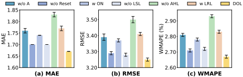
Figure 3 illustrates the effectiveness of each component in DOL. w/o A omits Awake phases; w/o Reset omits the SMB reset at the start of each Hibernate phase; w On replaces SUM with the online strategy from prior work [Pham et al., 2023], which updates the model with the latest observations; w/o LSL excludes LSL, updating the default ST network using SUM; w/o AHL excludes both SUM and LSL, using only the default ST network; w LRL replaces LSL with shared vanilla MLP layers across all locations.
The results indicate that: (1) w/o A underperforms methods with online strategies, e.g., w/o Reset, w On, and w/o LSL, highlighting the significance of the online setting in urban ST forecasting. (2) The inferior results of w/o Reset confirm our presumption that outdated samples are not relevant to current forecasting. (3) DOL outperforms w On, demonstrating that our SUM surpasses existing strategies by leveraging historical knowledge to mitigate catastrophic forgetting and introducing randomness to avoid overfitting. (4) w/o LSL and w/o AHL validate the effectiveness of our strategies for online urban ST forecasting. Notably, the degraded performance of w/o LSL shows that directly applying online strategies to traditional ST networks is inadequate, as they fail to adapt to location-specific shifts. (5) DOL achieves a 5.65% reduction in MAE compared to w LRL, confirming that updating the network without considering location-specific distributions is insufficient. By adapting to each location individually, DOL effectively handles locationspecific shifts. (6) Removing each component significantly degrades performance (𝑝 < 0.001), with MAE increasing by 1.80-9.58%, validating the necessity of all components.
5.6 Effects of Hyperparameters (RQ5)
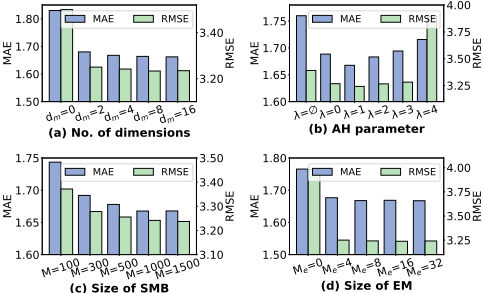
In Figure 4, we study the effects of hyperparameters in DOL. The results indicate that: (1) Increasing 𝑑𝑚 from 4 to 16 lowers MAE and RMSE by enhancing network capability, whereas 𝑑𝑚 = 0, which ignores location-specific shifts, significantly degrades performance, underscoring the importance of location-specific modeling. As DOL performs well with 𝑑𝑚 = 4, we select it as our default setting. (2) DOL performs best at 𝜆 = 1, with performance dropping as 𝜆 increases. Removing Awake phases (𝜆 = 0) significantly degrades performance, indicating that distribution shifts over time and requires online updates. Eliminating the Hibernate phases (𝜆 = ∅) also hurts performance, confirming the benefit of intermittent updates under gradual shifts. Surprisingly, even with an extended Hibernate phase (𝜆 = 2), DOL outperforms its no-Hibernate variant, implying overly frequent updates can lead to overfitting.
6 Conclusion
In this paper, we investigate the gradual and location-specific distribution shifts in urban ST streams and introduce DOL, a novel distribution-aware online learning framework for urban ST forecasting. DOL addresses gradual distribution shifts using a streaming update mechanism that intermittently pauses network updates, enabling adaptation with lower computational overhead. It handles location-specific shifts through an adaptive ST network with a location-specific learner, enabling adaptation to varying shifts across urban locations. These components can be seamlessly integrated into existing offline ST networks to enhance performance. Extensive experiments on four real-world datasets validate the effectiveness of DOL.
@inproceedings{ijcai2025p372,
  title     = {Distribution-Aware Online Learning for Urban Spatiotemporal Forecasting on Streaming Data},
  author    = {Wang, Chengxin and Tan, Gary and Barman Roy, Swagato and Ooi, Beng Chin},
  booktitle = {Proceedings of the Thirty-Fourth International Joint Conference on
               Artificial Intelligence, {IJCAI-25}},
  publisher = {International Joint Conferences on Artificial Intelligence Organization},
  editor    = {James Kwok},
  pages     = {3344--3352},
  year      = {2025},
  month     = {8},
  note      = {Main Track},
  doi       = {10.24963/ijcai.2025/372},
  url       = {https://doi.org/10.24963/ijcai.2025/372},
}
TY - CPAPER TI - Distribution-Aware Online Learning for Urban Spatiotemporal Forecasting on Streaming Data AU - Wang, Chengxin AU - Tan, Gary AU - Barman Roy, Swagato AU - Ooi, Beng Chin T2 - Proceedings of the Thirty-Fourth International Joint Conference on Artificial Intelligence, IJCAI-25 PB - International Joint Conferences on Artificial Intelligence Organization PY - 2025 SP - 3344 EP - 3352 DO - 10.24963/ijcai.2025/372 UR - https://doi.org/10.24963/ijcai.2025/372 ER -Copied
Machine-readable versions of this paper, for tools and AI agents:





