
ILIF: Temporal Inhibitory Leaky Integrate-and-Fire Neuron for Overactivation in Spiking Neural Networks
Proceedings of the Thirty-Fourth International Joint Conference on Artificial Intelligence. Main Track. Pages 4200-4208.
https://doi.org/10.24963/ijcai.2025/468
Keywords
- Machine Learning: ML: Other
- Machine Learning: ML: Representation learning
- Computer Vision: CV: Machine learning for vision
- Humans and AI: HAI: Cognitive modeling
Abstract
The Spiking Neural Network (SNN) has drawn increasing attention for its energy-efficient, event-driven processing and biological plausibility. To train SNNs via backpropagation, surrogate gradients are used to approximate the non-differentiable spike function, but they only maintain nonzero derivatives within a narrow range of membrane potentials near the firing threshold—referred to as the surrogate gradient support width gamma. We identify a major challenge, termed the dilemma of gamma: a relatively large gamma leads to overactivation, characterized by excessive neuron firing, which in turn increases energy consumption, whereas a small gamma causes vanishing gradients and weakens temporal dependencies. To address this, we propose a temporal Inhibitory Leaky Integrate-and-Fire (ILIF) neuron model, inspired by biological inhibitory mechanisms. This model incorporates interconnected inhibitory units for membrane potential and current, effectively mitigating overactivation while preserving gradient propagation. Theoretical analysis demonstrates ILIF’s effectiveness in overcoming the gamma dilemma, and extensive experiments on multiple datasets show that ILIF improves energy efficiency by reducing firing rates, stabilizes training, and enhances accuracy. The code is available at github.com/kaisun1/ILIF.
- [Bellec et al., 2018] Guillaume Bellec, Darjan Salaj, Anand Subramoney, Robert Legenstein, and Wolfgang Maass. Long short-term memory and learning-to-learn in net- works of spiking neurons. NeurIPS, 31, 2018.
- [Cai and Li, 2021] Zongyuan Cai and Xinze Li. Neuro- morphic brain-inspired computing with hybrid neural net- works. In 2021 IEEE International Conference on Artifi- cial Intelligence and Industrial Design (AIID), pages 343- 347. IEEE, 2021.
- [Dampfhoffer et al., 2022] Manon Dampfhoffer, Thomas Mesquida, Alexandre Valentian, and Lorena Anghel. In- vestigating current-based and gating approaches for ac- curate and energy-efficient spiking recurrent neural net- works. In International Conference on Artificial Neural Networks, pages 359-370. Springer, 2022.
- [Deng et al., 2023] Shikuang Deng, Hao Lin, Yuhang Li, and Shi Gu. Surrogate module learning: Reduce the gradi- ent error accumulation in training spiking neural networks. In ICML, pages 7645-7657. PMLR, 2023.
- [Ding et al., 2022] Jianchuan Ding, Bo Dong, Felix Heide, Yufei Ding, Yunduo Zhou, Baocai Yin, and Xin Yang. Bi- ologically inspired dynamic thresholds for spiking neural networks. NeurIPS, 35:6090-6103, 2022.
- [Duan et al., 2022] Chaoteng Duan, Jianhao Ding, Shiyan Chen, Zhaofei Yu, and Tiejun Huang. Temporal effective batch normalization in spiking neural networks. NeurIPS, 35:34377-34390, 2022.
- [Fang et al., 2020] Haowen Fang, Amar Shrestha, Ziyi Zhao, and Qinru Qiu. Exploiting neuron and synapse filter dy- namics in spatial temporal learning of deep spiking neural network. arXiv preprint arXiv:2003.02944, 2020. IJCAI
- [Fang et al., 2021a] Wei Fang, Zhaofei Yu, Yanqi Chen, Tiejun Huang, Timothée Masquelier, and Yonghong Tian. Deep residual learning in spiking neural networks. NeurIPS, 34:21056-21069, 2021.
- [Fang et al., 2021b] Wei Fang, Zhaofei Yu, Yanqi Chen, Timothée Masquelier, Tiejun Huang, and Yonghong Tian. Incorporating learnable membrane time constant to en- hance learning of spiking neural networks. ICCV, pages 2661-2671, 2021.
- [Guo et al., 2023] Yufei Guo, Yuhan Zhang, Yuanpei Chen, Weihang Peng, Xiaode Liu, Liwen Zhang, Xuhui Huang, and Zhe Ma. Membrane potential batch normalization for spiking neural networks. In ICCV, pages 19420-19430, 2023.
- [Huang et al., 2024] Yulong Huang, Xiaopeng Lin, Hongwei Ren, Haotian Fu, Yue Zhou, Zunchang Liu, Biao Pan, and Bojun Cheng. Clif: Complementary leaky integrate-and- fire neuron for spiking neural networks. ICML, 2024.
- [Jiang et al., 2024] Haiyan Jiang, Vincent Zoonekynd, Giu- lia De Masi, Bin Gu, and Huan Xiong. Tab: Temporal ac- cumulated batch normalization in spiking neural networks. In ICLR, 2024.
- [Li et al., 2021] Yuhang Li, Yufei Guo, Shanghang Zhang, Shikuang Deng, Yongqing Hai, and Shi Gu. Differen- tiable spike: Rethinking gradient-descent for training spik- ing neural networks. NeurIPS, 34:23426-23439, 2021.
- [Maass, 1997] Wolfgang Maass. Networks of spiking neu- rons: the third generation of neural network models. Neu- ral networks, 10(9):1659-1671, 1997.
- [Meng et al., 2023] Qingyan Meng, Mingqing Xiao, Shen Yan, Yisen Wang, Zhouchen Lin, and Zhi-Quan Luo. Towards memory-and time-efficient backpropagation for training spiking neural networks. In ICCV, pages 6166- 6176, 2023.
- [Neftci et al., 2019] Emre O Neftci, Hesham Mostafa, and Friedemann Zenke. Surrogate gradient learning in spik- ing neural networks: Bringing the power of gradient-based optimization to spiking neural networks. IEEE Signal Pro- cessing Magazine, 36(6):51-63, 2019.
- [Niu and Wei, 2023] Li-Ye Niu and Ying Wei. Cirm-snn: Certainty interval reset mechanism spiking neuron for en- abling high accuracy spiking neural network. Neural Pro- cessing Letters, 55(6):7561-7582, 2023.
- [Tavanaei et al., 2019] Amirhossein Tavanaei, Masoud Gho- drati, Saeed Reza Kheradpisheh, Timothée Masquelier, and Anthony Maida. Deep learning in spiking neural net- works. Neural networks, 111:47-63, 2019.
- [Wang and Yu, 2024] Lihao Wang and Zhaofei Yu. Autaptic synaptic circuit enhances spatio-temporal predictive learn- ing of spiking neural networks. PMLR, 2024.
- [Wei et al., 2023] Wenjie Wei, Malu Zhang, Hong Qu, Am- mar Belatreche, Jian Zhang, and Hong Chen. Temporal- coded spiking neural networks with dynamic firing thresh- old: Learning with event-driven backpropagation. In ICCV, pages 10552-10562, 2023.
- [Werbos, 1990] Paul J Werbos. Backpropagation through time: what it does and how to do it. Proceedings of the IEEE, 78(10):1550-1560, 1990.
- [Xiao et al., 2022] Mingqing Xiao, Qingyan Meng, Zong- peng Zhang, Di He, and Zhouchen Lin. Online train- ing through time for spiking neural networks. NeurIPS, 35:20717-20730, 2022.
- [Yao et al., 2022] Xingting Yao, Fanrong Li, Zitao Mo, and Jian Cheng. Glif: A unified gated leaky integrate-and-fire neuron for spiking neural networks. NeurIPS, 35:32160- 32171, 2022.
- [Zenke and Ganguli, 2018] Friedemann Zenke and Surya Ganguli. Superspike: Supervised learning in multi- layer spiking neural networks. Neural computation, 30(6):1514-1541, 2018.
- [Zhang et al., 2019] Anguo Zhang, Hongjun Zhou, Xiumin Li, and Wei Zhu. Fast and robust learning in spiking feed-forward neural networks based on intrinsic plasticity mechanism. Neurocomputing, 365:102-112, 2019.
- [Zheng et al., 2021] Hanle Zheng, Yujie Wu, Lei Deng, Yi- fan Hu, and Guoqi Li. Going deeper with directly-trained larger spiking neural networks. In AAAI, volume 35, pages 11062-11070, 2021.
References were extracted automatically from the PDF and may contain errors.
Full text extracted automatically from the PDF; figures, tables and equations may differ. The PDF is the version of record.
1 Introduction
The Spiking Neural Network (SNN), recognized as the third generation of neural networks, is distinguished by the simulation of neuronal message passing through spike-based activations [Maass, 1997]. Unlike the traditional Artificial Neural Network (ANN), which process information with continuous values, SNN, driven by the dynamic accumulation of membrane potential to trigger discrete activation events, effectively mimics the behavior of biological neurons by propagating discrete spike signals (0 or 1) between neurons [Tavanaei et al., 2019]. This spike-based processing endows SNN with remarkable energy efficiency, especially when deployed on neuromorphic hardware platforms such as Intel's Loihi, IBM's TrueNorth, and Tianjic chips [Cai and Li, 2021].
A key challenge in gradient-based optimization for training SNNs is its inherent non-differentiability due to the discrete nature of spike transmissions between neurons. To resolve this issue, surrogate gradient (SG) has been introduced to enable backpropagation in SNNs [Neftci et al., 2019]. However, these approximations can cause or worsen two major issues: overactivation and gradient vanishing. Specifically, overactivation occurs when the accumulated membrane potential surpasses twice the threshold, causing excessive spiking that drives up energy consumption and masks essential temporal information. Strategies such as adaptive thresholding, residual membrane potential modulation, and normalization have been proposed to regulate neuronal activity and mitigate overactivation [Wei et al., 2023; Wang and Yu, 2024; Jiang et al., 2024]. Gradient vanishing, on the other hand, stems from the mismatch between surrogate gradients and discrete spikes, as well as membrane potential decay, resulting in ineffective backpropagation. Current solutions, such as residual learning and adaptive mechanisms [Fang et al., 2021a; Yao et al., 2022], enhance gradient propagation and improve training efficiency.
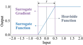
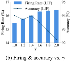
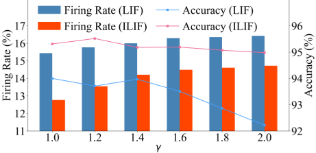
Existing research often treats overactivation and gradient vanishing as separate issues, overlooking the conflicting effects of the SG on both phenomena. As shown in Figure 1a, given the support width γ in the SG, Figure 1b demonstrates that a larger γ results in elevated firing rates and reduced accuracy (more details will be presented in Section 4.1). However, as [Huang et al., 2024] points out, when the threshold remains constant, a smaller γ risks gradient vanishing. In this paper, this contradiction is referred to as the dilemma of γ, which highlights the need to balance the mitigation of overactivation with the preservation of gradient flow. Inspired by the brain's efficient spike regulation through feedforward and feedback inhibition, which controls excessive activation, our objective is to design a module that mitigates the γ-induced conflict between overactivation and gradient vanishing.
This study conducts a theoretical examination of the relationship between γ and both excessive activation and the disappearance of gradients. To address the difficulty of balancing overactivation and gradient vanishing solely by adjusting γ, we propose a temporal Inhibitory Leaky Integrate-andFire (ILIF) neuron model with two inhibitory units, namely the membrane potential inhibitory unit (MPIU) and the current inhibitory unit (CIU), which are designed to mimic the
(a) Surrogate gradient
inhibitory mechanism of the human brain. The major contributions of this work are as follows:
- Theoretical Analysis: We conduct an in-depth mathematical investigation to clarify how the configuration of γ affects overactivation and its conflict with gradient vanishing, while analyzing how ILIF effectively mitigates both issues.
- SNN Modeling: The proposed MPIU and CIU in the ILIF neuron model function as feedforward and feedback inhibition, temporally interacting to reduce excessive activation and mitigate gradient vanishing.
- Experimental Validation: Comprehensive experiments demonstrate that the ILIF model's temporal inhibition mechanism generates fewer spikes while achieving a more stable training process and higher accuracy.
2 RelatedWork
2.1 Overactivation Control
To mitigate overactivation in SNN, prior works have proposed adaptive thresholds, residual potential modulation, and normalization. Adaptive threshold methods dynamically raise or lower the firing threshold based on recent activity patterns [Ding et al., 2022; Wei et al., 2023; Fang et al., 2020; Zhang et al., 2019]. Residual modulation methods, such as TC-LIF and CLIF, reduce post-spike membrane potential to suppress reactivation, mimicking the effect of afterhyperpolarization (AHP) [Wang and Yu, 2024; Niu and Wei, 2023]. Normalization techniques standardize input distributions across layers and time to stabilize spiking activity [Jiang et al., 2024; Guo et al., 2023; Duan et al., 2022]. However, these methods often rely on handcrafted rules or instantaneous signals, lacking temporal adaptability and biological interpretability. In contrast, our ILIF model integrates inhibitory units that accumulate both short- and long-term activity, and crucially, adjusts inhibition based on the post-spike membrane potential, providing more precise, causal, and biologically aligned suppression than methods like TC-LIF and CLIF, which depend on pre-spike estimates and risk over-inhibition.
2.2 Improving Gradient Propagation
Due to the intrinsic properties of spiking neurons-namely, spike-based activation and membrane potential decay-temporal gradients often vanish over time. A key factor contributing to this vanishing is the leakage of membrane potential, which diminishes the impact of earlier inputs as time progresses. To mitigate this, models such as PLIF [Fang et al., 2021b] adaptively adjust the leakage rate, preserving critical temporal information. Similarly, gating mechanisms employed in models like GLIF [Yao et al., 2022], STC-LIF [Wang and Yu, 2024], and SpikGRU [Dampfhoffer et al., 2022] enhance temporal dependencies by regulating information flow within neurons. However, these methods typically incur additional computational overhead and are limited to intra-neuron dynamics. In contrast, our approach introduces biologically inspired temporal connections between inhibitory units, serving as shortcuts that simultaneously facilitate backward gradient propagation and forward inhibitory signaling, thereby enhancing temporal dependencies without increasing model parameters.
3 Preliminary
3.1 Vanilla LIF NeuronModel
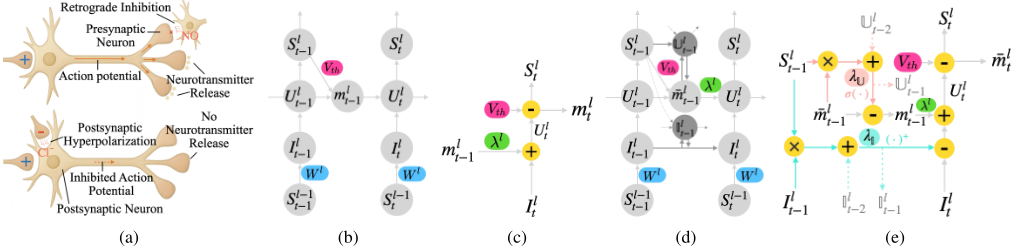
As shown in Figures 2b and 2c, the LIF serves as a fundamental computational framework, encompassing membrane potential integration, leakage, and spike firing upon exceeding the threshold. The model is described by the following equations:
In the LIF model, U l [t] is the membrane potential in the l-th layer at time step t, combining the postsynaptic current I l [t] and the residual membrane potential from the previous time step ml [t - 1] with a decay factor λ. The postsynaptic current I l [t] is computed as the product of the synaptic weight W l and the input spike Sl-1 [t]. The output spike Sl [t] is generated using the Heaviside function H(·), which outputs a spike (Sl [t] = 1) when the membrane potential U l [t] exceeds the threshold Vth and no spike (Sl [t] = 0) otherwise. After firing, the membrane potential ml [t] is softly reset by subtracting Vth.
3.2 Spatio-Temporal Backpropagation
Training SNN directly involves implementing Backpropagation Through Time (BPTT) [Werbos, 1990] and using SG to handle the non-differentiability of spike signals. The gradient of the loss function L with respect to the weight W l at layer l is calculated across all time steps T. It is given by
This gradient is computed by decomposing it into spatial and temporal components:
The Spatial Term represents the gradient contribution from the current time step, while the Temporal Term accounts for the influence of future time steps on the current gradient. It is calculated recursively as follows:
where the term ϵl [t] for LIF model is as:
Detailed derivations are provided in Appendix A. The derivative ∂Sl [t] ∂U l [t] is approximated with the SG H′ (U l [t]), where H(·) provides a smooth approximation of the Heaviside function. A common choice for the SG is the rectangular function, defined as:
where 1(·) is the indicator function, and γ controls the SG support width. γ is typically set to Vth [Meng et al., 2023]. In this case
The gradient ∂L ∂Sl [t] in Eq. (7) varies depending on the layers:
3.3 InhibitoryMechanism
In neural systems, various inhibitory mechanisms ensure stable and efficient signal processing. For instance, after a neuron fires an action potential, its membrane potential undergoes afterhyperpolarization. This causes the potential to drop below the resting level, reducing excitability and preventing immediate re-firing. The effect of afterhyperpolarization accumulates over successive spikes, intensifying suppression over time. Additionally, activated downstream neurons send retrograde inhibitory signals to presynaptic neurons by modulating ion channel activity and suppressing neurotransmitter release. This process, mediated by GABAergic interneurons and commonly referred to as retrograde inhibition, suppresses presynaptic currents and limits excessive signal transmission [Bellec et al., 2018; Zenke and Ganguli, 2018]. Inspired by these mechanisms, we enhance the LIF model by incorporating inhibitory processes to reduce overactivation and facilitate more effective gradient flow. The corresponding inhibitory mechanisms are illustrated in Figure 2a.
4 Methodology
4.1 The Dilemma of γ
The dilemma of γ refers to the challenge of balancing overactivation and gradient vanishing in neural networks. The correlation between γ and overactivation has been underexplored, motivating our investigation into this correlation.
Lemma 1. The likelihood of experiencing overactivation is positively correlated with γ.
Proof. When the neural network converges to an optimum such that no further weight updates occur, we consider the system to have reached an equilibrium. Let W1 be the equilibrium weights when γ = γ1 and W2 be the equilibrium weights when γ = γ2, with γ2 > γ1. Suppose that there are neurons in the firing state (requiring W lSl-1 [t] > 0 to accumulate sufficient membrane potential), whereas others remain inactive (requiring W lSl-1 [t] < 0 to suppress activation).
In the output layer, the gradient terms related to the loss function are: ∂L ∂SL [t] = Y L[t] - ˆ Y L[t], ∂U L [t] ∂W L = SL-1 [t], where Y L[t] represents the average output (within [0,1]), and ˆ Y L[t] represents the predicted values encoded in a one-hot format (taking values of either 0 or 1). As derived from Equations (5), (7), (9) and (10), the expected gradient with respect toW L is
Under the SG framework, the gradient for a given sample becomes zero whenever the membrane potential moves outside the range [Vth - γ2 , Vth + γ2 ]. Neurons whose membrane potentials exceed or fall below this interval stop receiving weight updates. As λ increases from λ1 to λ2, neurons previously outside the range may re-enter it, allowing further updates during the transition fromW1 toW2.
According to Equation (12), Neurons expected to fire ( ˆ Y [t′ ] = 1) receive negative gradients, which increase positive weights. Conversely, neurons expected to remain inactive ( ˆ Y [t′ ] = 0) receive positive gradients, which decrease negative weights. This process contributes to an overall increase in the weight norm ∥W∥. Additionally, based on Equation (11) and the chain rule, changes in the final layer's weights propagate to earlier layers, causing their weights to increase or decrease accordingly.
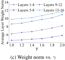
During activation, the membrane potential increment is W lSl-1 [t]. A larger ∥W∥ amplifies this increment, increasing the chance of exceeding twice the threshold and causing overactivation. As shown in Figure 1c, increasing γ leads to a higher average layer weight norm, which amplifies the membrane potential further, thereby heightening the risk of overactivation.
Lemma 2. The likelihood of experiencing gradient vanishing is inversely correlated with γ.
The gradient in Eq. (7) includes the product ∏ ϵl [t], where ϵl [t] = 1-Vth/γ when the membrane potential is near threshold and γ > Vth. As γ decreases toward Vth, this factor becomes smaller, reducing the gradient magnitude over time. At γ = Vth, ϵl [t] = 0, and gradients are completely blocked. See Appendix B for details.
As seen from Lemmas 1 and 2, the impact of γ is twofold: increasing γ exacerbates overactivation, while decreasing it increases the risk of gradient vanishing. This trade-off demonstrates the limitation of adjusting γ alone to improve SNN performance. Thus, specialized modules are needed to strike an optimal balance between these competing effects.
4.2 ILIF NeuronModel
To address overactivation and gradient vanishing in the vanilla LIF model, we propose the ILIF model with two biologically-inspired inhibitory mechanisms. The MPIU provides long-term inhibition by mimicking afterhyperpolarization, stabilizing neuronal excitability. The CIU delivers short-term inhibition via retrograde-like feedback, regulating presynaptic currents. The ILIF structure and internal operations are illustrated in Figures 2d and 2e.
MPIU Each spike contributes to the integration of the postspike membrane potential ¯ml [t] into Ul [t], which decays slowly (λU ≈ 1) to maintain a long-term memory of spiking activity:
This unit accumulates historical firing patterns, retaining the neuron's firing history and mimicking the afterhyperpolarization phenomenon in biological systems. As firing activity accumulates, the accumulated inhibition Ul [t] grows, progressively reducing excitability and preventing excessive firing. This inhibition directly affects the membrane potential before subsequent firings:
where σ(·) is a bounded sigmoid function that allows inhibition to increase with historical firing, in contrast to linear mappings or unbounded nonlinear functions that may lead to instability. This mirrors synaptic plasticity mechanisms that adjust synaptic strengths based on past activity, preventing excessive suppression and maintaining learnability over extended timescales. Moreover, the temporal linkage within MPIU mitigates vanishing gradients by offering a direct pathway for backpropagation, as further analyzed in Section 4.3.
CIU Complementing the MPIU's long-term inhibition, the CIU provides rapid, short-term feedback. With a decay coefficient λI close to 0, primarily inhibiting the incoming current based on the previous time step's current and the current spikes from the next layer:
The incoming current is adjusted as follows:
Here, Il [t - 1]+ ensures non-negative inhibition, mimicking the rapid feedback mediated by GABAergic interneurons in biological systems. By delivering rapid inhibition tied to the prior spikes and current, the CIU stabilizes excitability in tandem with MPIU.
Combining these mechanisms, the ILIF model evolves according to the following equations, with the corresponding pseudocode provided in Appendix E:
4.3 Analysis of the ILIFModel
The ILIF model builds directly upon the vanilla LIF model by introducing inhibitory decay factors λU and λI. Setting these factors to zero removes all inhibitory effects, reducing the ILIF model to the standard LIF model. This demonstrates that the ILIF model's inhibitory mechanisms are natural extensions that refine the neuron's behavior without altering its fundamental structure. In this analysis, we explore the relationship between the ILIF and LIF models and the underlying principles that enable the ILIF model to overcome the limitations of the LIF model.
Theorem 1. W ′ is the equilibriumweight in the vanilla LIF, and W ′′ is the new equilibrium weight in the ILIF, ∥W ′′ ∥> ∥W ′ ∥.
Proof. In the vanilla LIF model, the gradient of the loss L with respect to U l [t] consists of both a spatial and a temporal term (denoted as a(W), highlighted in blue). In contrast, the ILIF model introduces additional gradient terms (denoted as b(W), highlighted in red), as shown in Equation (18). A detailed derivation is provided in Appendix C.
where ϕl [t] encapsulates the derivatives associated with MPIU and CIU:
Consider the vanilla LIF model without inhibition, where the equilibrium weight W ′ satisfies a(W ′ ) = 0. The function a(W) includes terms that are products of W and typically oppose the sign of W. Introducing an additional gradient b(W), which shares the same sign as W (see Appendix D), modifies the total gradient to a(W)+b(W), and the new equilibriumW ′′ must satisfy a(W ′′ ) + b(W ′′ ) = 0.
If W ′′ > 0, then b(W ′′ ) > 0 and thus a(W ′′ ) < 0 to maintain equilibrium. Since a(W) becomes more negative as W increases, this implies W ′′ > W ′ . Similarly, if W ′′ < 0, then b(W ′′ ) < 0 and a(W ′′ ) > 0, and because a(W) becomes more positive as W decreases, it follows that W ′′ <W ′ .
Therefore, in both cases, the magnitude of the new equilibrium increases: ∥W ′′ ∥> ∥W ′ ∥. Empirical results supporting this conclusion are provided in Section 5.3.
Theorem 2. r′ is the equilibrium firing rate in the vanilla LIF, and r′′ is the new equilibrium firing rate in the ILIF. It satisfies that r′′ < r′ even ∥W ′′ ∥> ∥W ′ ∥.
Proof. According to Lemma 1, we define the excitatory input function F(∥W∥), which increases with ∥W∥, indicating that larger weight magnitudes result in higher excitatory input necessary for neuron firing, and the response function R(x), which maps input x to firing rate r, reflecting that higher inputs lead to increased activation. Additionally, based on Equations (13) and (15), we define the inhibition function J(r), which increases with the firing rate r and satisfies J(r) ≥ 0 for all r ≥ 0, ensuring that higher firing rates induce stronger inhibitory effects.
In the vanilla LIF without inhibition, the equilibrium firing rate is r′ = R(F(∥W ′ ∥)). When inhibition is introduced, the new equilibrium rate satisfies r′′ = R(F(∥W ′′ ∥) - J(r′′ )). By Theorem 1, we know that ∥W ′′ ∥> ∥W ′ ∥.
To prove r′′ < r′ , suppose instead that r′′ ≥ r′ . Since R is increasing, we have
which implies F (∥W ′′ ∥) - F (∥W ′ ∥) ≥ J(r′′ ) > 0. Define the function H(r) = R(F(∥W ′′ ∥) - J(r)). Since both R and J are strictly increasing, we have
so H(r) is strictly decreasing. Note that J(r′ ) = 0, so
By the fixed-point theorem 1 , since H(r′ ) > r′ and H is decreasing, the fixed point r′′ = H(r′′ ) must satisfy r′′ < r′ , contradicting our assumption.
Therefore, r′′ < r′ . This shows that even though ∥W ′′ ∥> ∥W ′ ∥, the resulting firing rate is strictly lower, meaning that inhibition effectively balances the excitatory input and prevents overactivation.
Theorem3. ILIF introduces additional gradient propagation pathways, mitigating the vanishing gradient problem.
1 Let f(x) be strictly decreasing. If f(x1) > x1, then any fixed point x∗ such that f(x∗ ) = x∗ must satisfy x∗ < x1.
Proof. According to Lemma 2, the vanishing gradient problem in LIF is caused by the term ϵl [t], which gradually accumulates to zero with lower γ. In ILIF, however, membrane potential inhibitory units introduce a direct shortcut that connects all time steps. Because each inhibitory unit is interconnected and the decay coefficient is set to 1 in our experiments, there exists a shortcut in the backward pass given by ∂Ul [t] ∂Sl [t] ∂Sl [t] ∂U l [t] enabling each time step's inhibitory unit to transmit the gradient directly to the preceding time step. Consequently, as inhibition stops after T with the output produced, the complete chain of partial derivatives from time step T -1 back to t can be written as:
Since there is no decay in these shortcuts, the gradient can flow from the time step T -1 back to any earlier step without attenuation. This mechanism mitigates the vanishing gradient problem and facilitates effective gradient propagation.
5 Experiments
5.1 Experimental Settings
In this research, we conduct experiments on two types of datasets without data augmentation: standard image classification datasets (CIFAR10 and CIFAR100) and neuromorphic datasets (DVSCIFAR10 and DVSGesture). For a comprehensive and unbiased evaluation, the proposed ILIF model is implemented under various settings, including different network architectures, neuron models, and training time steps. Further details are provided in Appendix F.
5.2 Evaluation of Accuracy
As shown in Table 1, our ILIF model consistently achieves superior top-1 accuracy compared to existing methods. Specifically, our method achieves 95.49% on CIFAR10 and 78.51% on CIFAR100 using the ResNet-18 architecture with 6 time-steps. For the neuromorphic dataset, ILIF achieves an accuracy of 78.60% on DVSCIFAR10 and matches the top-1 accuracy of 97.92% achieved by other models on DVSGesture, further demonstrating its effectiveness. More experiments are provided in Appendix J.
5.3 Effectiveness of Overactivation Inhibition
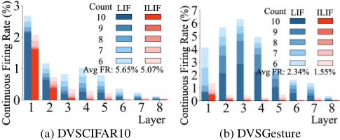
We quantified the proportion of neurons activated for more than half the time. As shown in Figure 4, the ILIF model consistently exhibits lower firing rates and fewer instances of continuous activation across all layers compared to LIF model on DVSCIFAR10 and DVSGesture. Furthermore, the reduction in continuous activation rates leads to a lower overall average firing rate, especially with the activation rate by over 30% on DVSGesture. Additional figures for all datasets are provided in the Appendix G.
To better understand the firing patterns across time steps and layers, we compared the spike counts of the LIF and ILIF
| Dataset | Method | Network Architecture | Time Step | Accuracy (%) |
|---|---|---|---|---|
| CIFAR10 | STBP-tdBN [Zheng et al., 2021] Dspike [Li et al., 2021] GLIF [Yao et al., 2022] SML [Deng et al., 2023] CLIF [Huang et al., 2024] Ours | ResNet-19 Modified ResNet-18 ResNet-18 ResNet-18 ResNet-18 ResNet-18 | 4 / 6 4 / 6 4 6 4 / 6 4 / 6 | 92.92 / 93.16 93.66 / 94.05 94.67 95.12 94.89 / 95.41 95.24 / 95.49 |
| CIFAR100 | STBP-tdBN [Zheng et al., 2021] Dspike [Li et al., 2021] GLIF [Yao et al., 2022] SML [Deng et al., 2023] CLIF [Huang et al., 2024] | ResNet-19 Modified ResNet-18 ResNet-18 ResNet-18 ResNet-18 | 4 / 6 4 / 6 4 / 6 6 | 70.86 / 71.12 73.35 / 74.24 76.42 / 77.28 78.00 |
| DVSCIFAR10 | Ours STBP-tdBN [Zheng et al., 2021] Dspike [Li et al., 2021] OTTT [Xiao et al., 2022] SLTT [Meng et al., 2023] | ResNet-18 ResNet-19 ResNet-18 VGG-11 | 4 / 6 4 / 6 10 | 77.00 / 78.36 77.43 / 78.51 67.8 75.40 |
| Ours | VGG-11 VGG-11 | 10 10 10 | 76.27 77.17 | |
| STBP-tdBN [Zheng et al., 2021] OTTT [Xiao et al., 2022] SLTT [Meng et al., 2023] CLIF [Huang et al., 2024] | ResNet-17 VGG-11 VGG-11 | 10 40 20 20 | 78.60 | |
| VGG-11 | 96.87 96.88 97.92 97.92 | |||
| 20 | ||||
| DVSGesture | ||||
| Ours | 20 | 97.92 | ||
| VGG-11 |
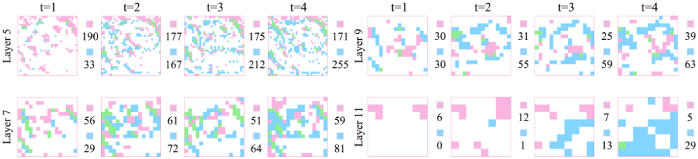
models. According to Theorems 1 and 2, inhibitory units lead to larger synaptic weights but also induce strong inhibition. As shown in Figure 3, the ILIF model exhibits a higher firing rate in the first time step due to the absence of immediate inhibition and larger synaptic weights. This efficiently captures critical information early, avoiding prolonged accumulation and delayed activation as observed in the LIF model, where the number of activations rises rapidly across time steps. In later time steps, firing rates decrease as inhibition suppresses redundant activations, ensuring efficient information transfer.
5.4 Evaluation of the Effect of γ on ILIF
Figure 5 illustrates the impact of varying γ on the firing rate and accuracy of the LIF and ILIF models. As γ increases, the LIF model experiences a significant decline in accuracy due to heightened activation, accompanied by a relatively higher firing rate. In contrast, the ILIF model consistently demonstrates a lower firing rate, highlighting its inhibitory effect.
| Settings | Accuracy (%) | ||||
|---|---|---|---|---|---|
| MPIU | CIU | CIFAR10 | CIFAR100 | DVS-C10 | DVS-Ges |
| ✓ | ✓ | 95.49 | 78.51 | 78.60 | 97.92 |
| ✓ | ✗ | 95.11 | 78.06 | 78.21 | 97.56 |
| ✗ | ✓ | 94.63 | 76.84 | 77.13 | 97.22 |
| ✗ | ✗ | 93.76 | 75.46 | 75.50 | 96.88 |
| Method CIFAR10 CIFAR100 DVS-C10 | DVS-Ges | |||
|---|---|---|---|---|
| PLIF | 94.25 | 75.65 | 75.32 | 95.49 |
| IPLIF | 95.61 | 78.66 | 78.41 | 96.55 |
Furthermore, the ILIF model works synergistically with the backpropagation shortcut provided by its inhibitory units, ensuring more stable accuracy across all γ values.
5.5 Ablation Study
We performed ablation experiments to evaluate the contributions of each inhibitory unit in the ILIF model. As shown in Table 2, removing either unit results in a noticeable drop in accuracy, confirming their necessity. To explore the generalizability of our proposed inhibitory mechanism, we integrated it into the PLIF model [Fang et al., 2021b], a LIF variation that adjusts decay parameters. This integration (Table 3) significantly enhances performance, demonstrating the value of our inhibitory mechanism given that PLIF only modifies decay parameters and inherits the limitations of LIF neurons.
6 Conclusion
This paper analyzes the limitations of the LIF model, specifically overactivation and gradient vanishing caused by the SG support width γ. Inspired by biological inhibitory mechanisms, we propose the ILIF model, which integrates MPIU and CIU to regulate neural activity and enhance gradient propagation simultaneously. Experiments show that ILIF achieves state-of-the-art performance, reduces continuous firing rates, and enhances result stability, providing an efficient and reliable solution for advancing neuromorphic computing.
Ethical Statement
There are no ethical issues.
Acknowledgments
This work was supported in part by start-up funds (No. MSRI8001004 and No. MSRI9002005), as well as by Monash eResearch capabilities, including M3.
@inproceedings{ijcai2025p468,
  title     = {ILIF: Temporal Inhibitory Leaky Integrate-and-Fire Neuron for Overactivation in Spiking Neural Networks},
  author    = {Sun, Kai and Duan, Peibo and Kuhlmann, Levin and Wang, Beilun and Zhang, Bin},
  booktitle = {Proceedings of the Thirty-Fourth International Joint Conference on
               Artificial Intelligence, {IJCAI-25}},
  publisher = {International Joint Conferences on Artificial Intelligence Organization},
  editor    = {James Kwok},
  pages     = {4200--4208},
  year      = {2025},
  month     = {8},
  note      = {Main Track},
  doi       = {10.24963/ijcai.2025/468},
  url       = {https://doi.org/10.24963/ijcai.2025/468},
}
TY - CPAPER TI - ILIF: Temporal Inhibitory Leaky Integrate-and-Fire Neuron for Overactivation in Spiking Neural Networks AU - Sun, Kai AU - Duan, Peibo AU - Kuhlmann, Levin AU - Wang, Beilun AU - Zhang, Bin T2 - Proceedings of the Thirty-Fourth International Joint Conference on Artificial Intelligence, IJCAI-25 PB - International Joint Conferences on Artificial Intelligence Organization PY - 2025 SP - 4200 EP - 4208 DO - 10.24963/ijcai.2025/468 UR - https://doi.org/10.24963/ijcai.2025/468 ER -Copied
Machine-readable versions of this paper, for tools and AI agents:





