
Long-Term Individual Causal Effect Estimation via Identifiable Latent Representation Learning
Proceedings of the Thirty-Fourth International Joint Conference on Artificial Intelligence. Main Track. Pages 4788-4796.
https://doi.org/10.24963/ijcai.2025/533
Keywords
- Knowledge Representation and Reasoning: KRR: Causality
- Machine Learning: ML: Causality
Abstract
Estimating long-term causal effects by combining long-term observational and short-term experimental data is a crucial but challenging problem in many real-world scenarios. In existing methods, several ideal assumptions, e.g. latent unconfoundedness assumption or additive equi-confounding bias assumption, are proposed to address the latent confounder problem raised by the observational data. However, in real-world applications, these assumptions are typically violated which limits their practical effectiveness. In this paper, we tackle the problem of estimating the long-term individual causal effects without the aforementioned assumptions. Specifically, we propose to utilize the natural heterogeneity of data, such as data from multiple sources, to identify latent confounders, thereby significantly avoiding reliance on idealized assumptions. Practically, we devise a latent representation learning-based estimator of long-term causal effects. Theoretically, we establish the identifiability of latent confounders,
with which we further achieve long-term effect identification. Extensive experimental studies, conducted on multiple synthetic and semi-synthetic datasets, demonstrate the effectiveness of our proposed method.
- [Almond et al., 2005] Douglas Almond, Kenneth Y Chay, and David S Lee. The costs of low birth weight. The Quar- terly Journal of Economics, 120(3):1031-1083, 2005.
- [Athey et al., 2019] Susan Athey, Raj Chetty, Guido W Im- bens, and Hyunseung Kang. The surrogate index: Com- bining short-term proxies to estimate long-term treatment effects more rapidly and precisely. Technical report, Na- tional Bureau of Economic Research, 2019.
- [Athey et al., 2020] Susan Athey, Raj Chetty, and Guido Im- bens. Combining experimental and observational data to estimate treatment effects on long term outcomes. arXiv preprint arXiv:2006.09676, 2020.
- [Cai et al., 2024] Ruichu Cai, Weilin Chen, Zeqin Yang, Shu Wan, Chen Zheng, Xiaoqing Yang, and Jiecheng Guo. Long-term causal effects estimation via latent surrogates representation learning. Neural Networks, 176:106336, 2024.
- [Cai et al., 2025] Ruichu Cai, Zhifan Jiang, Kaitao Zheng, Zijian Li, Weilin Chen, Xuexin Chen, Yifan Shen, Guangyi Chen, Zhifeng Hao, and Kun Zhang. Learning disentangled representation for multi-modal time-series sensing signals. In Proceedings of the ACM on Web Con- ference 2025, WWW '25, page 3247-3266, New York, NY, USA, 2025. Association for Computing Machinery.
- [Chen and Ritzwoller, 2023] Jiafeng Chen and David M Ritzwoller. Semiparametric estimation of long-term treat- ment effects. Journal of Econometrics, 237(2):105545, 2023.
- [Chen et al., 2025a] Weilin Chen, Ruichu Cai, Junjie Wan, Zeqin Yang, and José Miguel Hernández-Lobato. Nonparametric heterogeneous long-term causal ef- fect estimation via data combination. arXiv preprint arXiv:2502.18960, 2025.
- [Chen et al., 2025b] Weilin Chen, Ruichu Cai, Yuguang Yan, Zhifeng Hao, and José Miguel Hernández-Lobato. Long-term causal inference via modeling sequential latent confounding. arXiv preprint arXiv:2502.18994, 2025.
- [Cheng et al., 2021] Lu Cheng, Ruocheng Guo, and Huan Liu. Long-term effect estimation with surrogate represen- tation. In Proceedings of the 14th ACM International Con- ference on Web Search and Data Mining, pages 274-282, 2021.
- [Chetty et al., 2011] Raj Chetty, John N Friedman, Nathaniel Hilger, Emmanuel Saez, Diane Whitmore Schanzenbach, and Danny Yagan. How does your kindergarten classroom affect your earnings? evidence from project star. The Quarterly journal of economics, 126(4):1593-1660, 2011.
- [Chung et al., 2015] Junyoung Chung, Kyle Kastner, Lau- rent Dinh, Kratarth Goel, Aaron C Courville, and Yoshua Bengio. A recurrent latent variable model for sequential data. Advances in neural information processing systems, 28, 2015.
- [Fleming et al., 1994] Thomas R Fleming, Ross L Prentice, Margaret S Pepe, and David Glidden. Surrogate and aux- iliary endpoints in clinical trials, with potential applica- tions in cancer and aids research. Statistics in medicine, 13(9):955-968, 1994.
- [Frangakis and Rubin, 2002] Constantine E Frangakis and Donald B Rubin. Principal stratification in causal infer- ence. Biometrics, 58(1):21-29, 2002.
- [Ghassami et al., 2022] AmirEmad Ghassami, Alan Yang, David Richardson, Ilya Shpitser, and Eric Tchetgen Tch- etgen. Combining experimental and observational data for identification and estimation of long-term causal effects. arXiv preprint arXiv:2201.10743, 2022.
- [Gregor et al., 2015] Karol Gregor, Ivo Danihelka, Alex Graves, Danilo Rezende, and Daan Wierstra. Draw: A recurrent neural network for image generation. In Interna- tional conference on machine learning, pages 1462-1471. PMLR, 2015.
- [Hill, 2011] Jennifer L Hill. Bayesian nonparametric mod- eling for causal inference. Journal of Computational and Graphical Statistics, 20(1):217-240, 2011.
- [Hohnhold et al., 2015] Henning Hohnhold, Deirdre O'Brien, and Diane Tang. Focusing on the long-term: It's good for users and business. In Proceedings of the 21th ACM SIGKDD International Conference on Knowledge Discovery and Data Mining, pages 1849-1858, 2015.
- [Hu et al., 2022] Wenjie Hu, Xiaohua Zhou, and Peng Wu. Identification and estimation of treatment effects on long- term outcomes in clinical trials with external observational data. arXiv preprint arXiv:2208.10163, 2022.
- [Hyvarinen and Morioka, 2016] Aapo Hyvarinen and Hi- roshi Morioka. Unsupervised feature extraction by time- contrastive learning and nonlinear ica. Advances in neural information processing systems, 29, 2016.
- [Imbens et al., 2024] Guido Imbens, Nathan Kallus, Xiaojie Mao, and Yuhao Wang. Long-term causal inference under persistent confounding via data combination. Journal of the Royal Statistical Society Series B: Statistical Method- ology, page qkae095, 2024.
- [Johansson et al., 2022] Fredrik D Johansson, Uri Shalit, Nathan Kallus, and David Sontag. Generalization bounds and representation learning for estimation of potential out- comes and causal effects. Journal of Machine Learning Research, 23(166):1-50, 2022.
- [Kallus and Mao, 2024] Nathan Kallus and Xiaojie Mao. On the role of surrogates in the efficient estimation of treat- ment effects with limited outcome data. Journal of the Royal Statistical Society Series B: Statistical Methodol- ogy, page qkae099, 2024.
- [Khemakhem et al., 2020] Ilyes Khemakhem, Diederik Kingma, Ricardo Monti, and Aapo Hyvarinen. Variational autoencoders and nonlinear ica: A unifying framework. In International Conference on Artificial Intelligence and Statistics, pages 2207-2217. PMLR, 2020.
- [Kingma and Welling, 2014] Diederik P. Kingma and Max Welling. Auto-encoding variational bayes. In Yoshua Ben- gio and Yann LeCun, editors, 2nd International Confer- ence on Learning Representations, ICLR 2014, Banff, AB, Canada, April 14-16, 2014, Conference Track Proceed- ings, 2014.
- [Kong et al., 2022] Lingjing Kong, Shaoan Xie, Weiran Yao, Yujia Zheng, Guangyi Chen, Petar Stojanov, Victor Akin- wande, and Kun Zhang. Partial disentanglement for do- main adaptation. In International conference on machine learning, pages 11455-11472. PMLR, 2022.
- [Künzel et al., 2019] Sören R Künzel, Jasjeet S Sekhon, Pe- ter J Bickel, and Bin Yu. Metalearners for estimat- ing heterogeneous treatment effects using machine learn- ing. Proceedings of the national academy of sciences, 116(10):4156-4165, 2019.
- [Lauritzen et al., 2004] Steffen L Lauritzen, Odd O Aalen, Donald B Rubin, and Elja Arjas. Discussion on causal- ity [with reply]. Scandinavian Journal of Statistics, 31(2):189-201, 2004.
- [Li et al., 2023] Zijian Li, Ruichu Cai, Guangyi Chen, Boyang Sun, Zhifeng Hao, and Kun Zhang. Sub- space identification for multi-source domain adaptation. Advances in Neural Information Processing Systems, 36:34504-34518, 2023.
- [Louizos et al., 2017] Christos Louizos, Uri Shalit, Joris M Mooij, David Sontag, Richard Zemel, and Max Welling. Causal effect inference with deep latent-variable models. Advances in neural information processing systems, 30, 2017.
- [Pearl, 2009] Judea Pearl. Causality. Cambridge university press, 2009.
- Ross L Prentice. Surrogate endpoints in clinical trials: definition and operational criteria. Statis- tics in medicine, 8(4):431-440, 1989.
- [Rubin, 1974] Donald B Rubin. Estimating causal effects of treatments in randomized and nonrandomized studies. Journal of educational Psychology, 66(5):688, 1974.
- [Singh, 2022] Rahul Singh. Generalized kernel ridge regres- sion for long term causal inference: Treatment effects, dose responses, and counterfactual distributions. arXiv preprint arXiv:2201.05139, 2022.
- [Wu and Fukumizu, 2022] Pengzhou Abel Wu and Kenji Fukumizu. β-intact-vae: Identifying and estimating causal effects under limited overlap. In International Conference on Learning Representations, 2022.
- [Wu et al., 2024] Peng Wu, Ziyu Shen, Feng Xie, Wang Zhongyao, Chunchen Liu, and Yan Zeng. Policy learn- ing for balancing short-term and long-term rewards. In Ruslan Salakhutdinov, Zico Kolter, Katherine Heller, Adrian Weller, Nuria Oliver, Jonathan Scarlett, and Fe- lix Berkenkamp, editors, Proceedings of the 41st Inter- national Conference on Machine Learning, volume 235 of Proceedings of Machine Learning Research, pages 53817-53846. PMLR, 21-27 Jul 2024.
- [Xu et al., 2023] Ziqi Xu, Debo Cheng, Jiuyong Li, Jixue Liu, Lin Liu, and Ke Wang. Disentangled representation for causal mediation analysis. In Proceedings of the AAAI Conference on Artificial Intelligence, volume 37, pages 10666-10674, 2023.
- [Xu et al., 2024] Ziqi Xu, Debo Cheng, Jiuyong Li, Jixue Liu, Lin Liu, and Kui Yu. Causal inference with con- ditional front-door adjustment and identifiable variational autoencoder. In The Twelfth International Conference on Learning Representations, ICLR 2024, Vienna, Austria, May 7-11, 2024. OpenReview.net, 2024.
- [Yang et al., 2024a] Qinwei Yang, Xueqing Liu, Yan Zeng, Ruocheng Guo, Yang Liu, and Peng Wu. Learning the optimal policy for balancing short-term and long-term re- wards. Advances in Neural Information Processing Sys- tems, 37:36514-36540, 2024.
- [Yang et al., 2024b] Zeqin Yang, Weilin Chen, Ruichu Cai, Yuguang Yan, Zhifeng Hao, Zhipeng Yu, Zhichao Zou, Zhen Peng, and Jiecheng Guo. Estimating long-term het- erogeneous dose-response curve: Generalization bound leveraging optimal transport weights. arXiv preprint arXiv:2406.19195, 2024.
- [Zhang et al., 2021] Weijia Zhang, Lin Liu, and Jiuyong Li. Treatment effect estimation with disentangled latent fac- tors. In Proceedings of the AAAI Conference on Artificial Intelligence, pages 10923-10930, 2021.
- [Zheng et al., 2025] Jiabi Zheng, Weilin Chen, Zhiyong Lin, Aqing Yang, and Zhifeng Hao. Long-term causal effects estimation across domains: an invariant surrogate repre- sentation learning approach. International Journal of Ma- chine Learning and Cybernetics, pages 1-13, 2025.
References were extracted automatically from the PDF and may contain errors.
Full text extracted automatically from the PDF; figures, tables and equations may differ. The PDF is the version of record.
1 Introduction
Estimating long-term causal effects is of increasing importance in many domains, such as healthcare, public education, marketing, and public policy [Hohnhold et al., 2015; Chetty et al., 2011; Fleming et al., 1994; Zheng et al., 2025]. In such long-term scenarios, it is usually difficult to conduct randomized control experiments to estimate the causal effects. Hence, a lot of researchers resort to the more easily accessible long-term observations. However, methods based on observational data still suffer from the latent confounding bias problem. Therefore, combining observational data and experimental data has emerged as a promising solution for estimating long-term causal effects [Imbens et al., 2024; Ghassami et al., 2022; Hu et al., 2022].
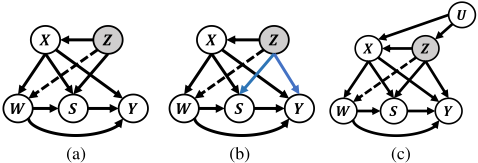
Existing data combination-based methods estimate longterm effects mainly based on the so-called surrogate. As shown in Fig. 1, the surrogate S is the short-term outcome, serving as the supplement or replacement for the long-term outcome Y in observational data. However, the unconfoundedness assumption is usually violated in such observational data due to the existence of latent confounders Z. As a replacement for unconfoundedness assumption, [Athey et al., 2020] propose an assumption named latent unconfoundedness, i.e., Y (w) ⊥ W|X, S(w) on observational data, implicitly indicating the latent confounders Z cannot affect longterm outcome Y as illustrated in Fig. 1a. Alternatively, to relax the unconfoundedness assumption, [Ghassami et al., 2022] introduces the (conditional) additive equi-confounding bias assumption, i.e., the magnitude of the confounding bias for the short-term and the long-term potential outcome variables are the same, as illustrated in Fig. 1b.
Existing methods, however, encounter a key challenge: the ideal assumptions are usually violated in real-world applications, including both the latent unconfoundedness and additive equi-confounding bias assumptions, which limit their practical effectiveness. For example, in studying the effect of driver income (treatment W) on long-term retention (outcome Y ) in a ride-hailing platform, driver characteristics (pre-treatment variable X) act as observed confounders affecting both income and retention. However, the drivers' household expenses (latent confounders Z) may also affect drivers' long-term retention Y , violating the latent unconfoundedness assumption. Similarly, the additive equiconfounding bias assumption may be violated since household expenses can influence short- and long-term retention differently, i.e., the confounding bias varies over time rather than remaining constant. Therefore, the strong assumptions in existing methods still significantly limit their applicability.
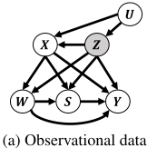
To address the above challenge, we aim to develop a method without the above assumptions to estimate the individual long-term causal effects as shown in Fig. 2. Specifically, instead of assuming latent unconfoundedness or equiconfounding bias, we explore the identifiability of latent confounders Z to estimate long-term causal effects. To identify latent confounder Z, we resort to an additional auxiliary variable U, which is easily accessible from our readily available prior knowledge, such as the natural heterogeneity of data in real-world applications. Recall the aforementioned drivers' income study example, the data are usually collected from various cities, and the indicator variable of the city can be directly taken as the auxiliary variable. Leveraging the identifiability of Z, we establish the causal effect identification result and propose the corresponding latent representation learningbased estimator for long-term individual causal effects. Overall, our contributions can be summarized as follows:
- We focus on a more general setting for estimating long-term causal effects, as shown in Fig. 1c. As shown in Fig. 1c, the assumed causal graph in our paper is a complete graph, and the causal graphs in existing work [Athey et al., 2020; Ghassami et al., 2022] can be seen as our special cases.
- We theoretically achieve the identifiability of latent confounders. Leveraging the identifiability result, we further establish the identification of long-term individual effects.
- We devise a latent representation learning-based estimator for effect estimation. The effectiveness of our estimator is verified on five synthetic and two real-world datasets. 1
2 RelatedWorks
Variational Auto-encoders for Causal Inference Variational Auto-encoder (VAE) [Kingma and Welling, 2014] is a powerful tool to capture latent structure in different kinds of applications, e.g., image processing [Gregor et al., 2015] and time-series [Chung et al., 2015; Cai et al., 2025]. In causal inference, VAE is used to recover unobserved variables to achieve the identification and estimation of the effects. Without unconfoundedness assumption, CEVAE [Louizos et al., 2017] assumes that latent confounders can be recovered by their proxies and applies VAE to learn confounders. As a follow-up work, TEDVAE [Zhang et al., 2021] and DMAVAE [Xu et al., 2023] decouple the learned latent confounders into several factors to achieve a more accurate estimation of treatment effects in different settings. With the recent development of VAE, nonlinear independent component analysis theory [Hyvarinen and Morioka, 2016] enables the identifiability of recovered variables, e.g., iVAE [Khemakhem et al., 2020] and SIG [Li et al., 2023]. CFDiVAE [Xu et al., 2024] apply iVAE to recover the front-door adjustment variable, achieving effect identification under the front-door criterion [Pearl, 2009]. β-Intact-VAE [Wu and Fukumizu, 2022] utilizes iVAE to recover prognostic scores to estimate effects under a limited overlap setting. Different from them, we achieve long-term individual effect identification and estimation by applying iVAE to recover the latent confounders.
1 The extended version is available at http://arxiv.org/abs/2505. 05192.
Long-term Causal Inference For decades, many works have explored what a valid surrogate is that can reliably predict long-term causal effects. Different types of criteria are proposed, e.g., prentice criteria [Prentice, 1989] and so on [Frangakis and Rubin, 2002; Lauritzen et al., 2004]. Recently, many works have explored estimating long-term causal effects based on surrogates via data combination. Under the unconfoundedness assumption, LTEE [Cheng et al., 2021] and Laser [Cai et al., 2024] are based on different designed neural networks for long-term causal inference. EETE [Kallus and Mao, 2024] studies the data efficiency from the surrogate and proposes efficient treatment effect estimation. Some works [Wu et al., 2024; Yang et al., 2024a] also focus on balancing short- and long-term rewards under the unconfoundedness assumption. Under surrogacy assumption, SInd [Athey et al., 2019] constructs the Surrogate Index as the substitutions for long-term outcomes in the experimental data to achieve effect identification and [Singh, 2022] propose a kernel ridge regression-based estimator for long-term effect under continuous treatment. As follow-up work, [Athey et al., 2020] assumes latent unconfoundedness assumption, i.e., short-term potential outcomes can mediate the long-term potential outcomes, to identify long-term causal effects. Under this assumption, several methods [Yang et al., 2024b; Chen and Ritzwoller, 2023] are proposed to estimate longterm effects more accurately. Other feasible assumptions are proposed to replace the latent unconfoundedness assumption, e.g., the additive equi-confounding bias assumption [Ghassami et al., 2022; Chen et al., 2025a] and its variant [Chen et al., 2025b]. Based on proximal methods, the sequential structure surrogates are studied [Imbens et al., 2024]. Different from them, we focus on estimating long-term individual causal effects in a more general scenario as shown in Fig. 1c.
3 ProblemDefinition
3.1 Notations
Our notations follow the potential outcome framework [Rubin, 1974]. Let W ∈ {0, 1} be a binary treatment variable. Let d◦ be the dimension of variable ◦. Let X ∈ X ⊆ Rdx
(b) Experimental data
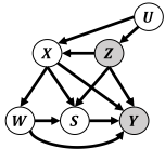
Figure 2: Two causal graphs in our setting. The white nodes denote observed variables and the grey nodes denote unobserved variables. Fig. 2a is the causal graph of observational data in our setting. Fig. 2b is the causal graph of experimental data in our setting.
be pre-treatment variable, Z ∈ Z ⊆ Rdz be latent confounders, S ∈ S ⊆ Rds be the short-term outcome variable, Y ∈ Y ⊆ R be the long-term outcome variable, and U ∈ U ⊆ Rdu be the auxiliary variable. Further, we denote the potential short-term outcomes S(w) ∈ Rds and potential long-term outcomes Y (w) ∈ R. Denote G ∈ {o, e} be the indicator of the data group, where G = o indicates the observational data, and G = e indicates the experimental data. Let lowercase letters (e.g., x, y) denote the value of random variables. Let lowercase letters with superscript (i) denote the value of the specified i-th unit. Following existing work [Athey et al., 2020; Hu et al., 2022; Ghassami et al., 2022], we consider the data combination setting. We have two types of data: the experimental data Dexp = {x(i) ,w(i) , s(i) , u(i) , g(i) = e}ne i=1 and the observational data Dobs = {x(i ,w(i) , s(i) , y(i) , u(i) , g(i) = o}no i=1+ne , where ne, no are the sample sizes of experimental and observational data respectively. Our setting is described in Fig. 2.
3.2 Assumptions and Target Estimands
Throughout this paper, we make the following assumptions: Assumption 1 (Long-term Effect Identification Assumptions). [Athey et al., 2020; Ghassami et al., 2022]
- A1 [Consistency, Positivity] If W = w, then Y = Y (w) and S = S(w). ∀w, x, 0 < P(W = w|X = x) < 1, 0 < P(G = o|W = w,X = x) < 1.
- A2 [Weak internal validity of observational data] for all w ∈ {0, 1}, W⊥⊥{Y (w), S(w)}|X, Z, G = o.
- A3 [Internal validity of experimental data] for all w ∈ {0, 1}, W⊥⊥{Y (w), S(w)}|X, G = e.
- A4 [External validity of experimental data] for all w ∈ {0, 1}, G⊥⊥{Y (w), S(w)}|X.
The assumptions above are mild and widely used in existing literature, e.g., [Athey et al., 2020; Ghassami et al., 2022]. A1 is a standard assumption. A2 allows the existence of latent confounders Z. A3 guarantees that the experimental data is unconfounded conditioned on X. A4 allows us to generalize the conditional distribution of potential outcomes between observational and experimental data.
In this paper, our task is to estimate the long-term individual treatment effects (ITE) given Dexp, Dobs, defined as:
as well as long-term average treatment effects (ATE), defined as:
4 Methodology
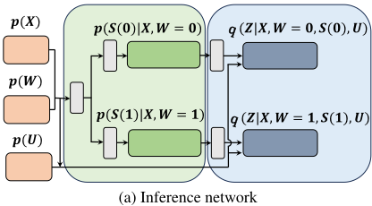
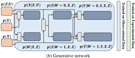
In this section, we present our end-to-end long-term causal effect estimator. Overall, as shown in Fig. 3, our estimator consists of three modules: short-term potential outcome estimation, latent representation learning, and ITE estimation. In the short-term potential outcome estimation module, we train an estimator for p(S(w)|W,X) using experimental data, as it is identifiable as p(S|W,X). In the latent representation learning module, we leverage variational inference to learn the latent representation of confounders Z. The pre-treatment variable X, treatment W and the short-term potential outcome S(w), obtained from the short-term potential outcome estimation module, are jointly treated as proxies for Z, ensuring sufficient information is available to recover Z. Additionally, the auxiliary variable U is used as a prior, guaranteeing the identifiability of the latent confounder Z, as demonstrated in the theoretical analysis (see Section 5).
In the ITE estimation module, based on learned Z, we conduct an estimator to learn the potential outcomes in treated and control groups, resulting in the final estimator of τ(x). Note that the first module is trained on experimental data to ensure the identification of short-term potential outcomes, and the others are trained on observational data since the long-term outcome is only observed in observational data.
4.1 Short-termPotential Outcome Estimation
We employ a multilayer perceptron (MLP) to model the distribution of p(S(w)|X) as our short-term potential outcome estimator. Since we can access short-term experimental data, p(S(w)|X) can be rewritten as p(S|X,W = w) on experimental data. To estimate that, inspired by Tarnet [Johansson et al., 2022], we use two heads of MLP for the estimation. Specifically, we can model each dimension of S(w) as a Gaussian distribution as follows:
where ˆµSi and ˆσSi are the mean and variance of the Gaussian distribution parametrized by the MLPs. We use the negative log-likelihood of Eq. (3) as the objective function LS(w) for the short-term potential outcome estimator as follows:
where qDexp is the empirical data distribution given by Dexp.
4.2 Latent Representation Learning
In the latent representation learning step, we employ iVAE to recover latent confounders Z, as shown in Fig. 3. This module consists of two networks: an inference network and a generative network. Specifically, for the inference network, the auxiliary variable U serves as additional information and thus our prior distribution is p(Z|U). We further use the posterior distribution q(Z|S(1), S(0),X,W,U) to approximate the prior, where the short-term potential outcomes are obtained by the short-term potential outcome estimator discussed in the previous section. For the generative network, we reconstruct the treatment W, the short-term outcome S and the pre-treatment covariate X.
Following exiting VAE-based works [Louizos et al., 2017], we choose the prior p(Z|U) as Gaussian distribution:
where ˆµi and ˆσi are the mean and variance of the Gaussian distribution parametrized by the MLPs.
To approximate the prior, we model the posterior distribution q(Z|S(1), S(0), X, W, U) as Gaussian distribution:
where ˆµZi|W=0 and ˆσZi|W=0 are the mean and variance of the Gaussian distribution parametrized by MLPs whose inputs are X,W,U and estimated S(W), and similarly for ˆµZi|W=1 and ˆσZi|W=1.
In the generative network, for a continuous variable, we parametrize the distribution as a Gaussian with its mean and variance both given by MLPs. For a binary variable, we use a Bernoulli distribution parametrized by an MLP similarly. Thus, we employ the following distributions for p(X|Z, U):
where ˆµXi and ˆσXi are the mean and variance of the Gaussian distribution parametrized by MLPs in the generative network when the variable is continuous, and ˆπXi is the mean of Bernoulli distribution parametrized by the generative network when the variable is binary. Similarly, we employ the following distributions for p(W|X, Z) and p(S|W, X, Z):
where ˆµS′i , ˆσS′i , ˆπS′i and ˆπWi are all parametrized by the generative network. We then use the negative variational Evidence Lower Bound (ELBO) as the objective function for the inference and generative networks (see Appendix E for the derivations):
where qDobs is the empirical data distributions given by Dobs.
4.3 ITE Estimation
To obtain the outcome Y , we introduce an auxiliary distribution that helps predict long-term outcome Y . Specifically, we employ the following distribution for p(Y |W, S, X, Z):
where ˆµyi and ˆσyi are the mean and variance of the Gaussian distribution parametrized by MLPs. We then use the negative log-likelihood as its objective function:
Overall, our final objective function L is
As a result, after training our method on experimental and observational data, given specific unit x(i) , u(i) , our final estimator yields long-term potential outcomes ˆ y(1)(i) , ˆ y(0)(i) on the treated and control group respectively. Thus the estimated long-term individual effect of x(i) , u(i) is
5 Theoretical Analysis
In this section, we present the identifiability result of our model and the identification of long-term individual causal effects. If we can correctly identify the latent confounders Z, the long-term individual causal effect can be identified based on the learned representation of Z. We first prove that Z is identifiable up to a simple transformation. Leveraging the identifiability result of Z, we further prove that the long-term individual causal effect is identifiable.
5.1 Identifiability of Latent Confounders
To clearly introduce the latent confounders identifiability result, we first denote Zi as the i-th dimension of Z. The identifiability of latent confounders means that, for each groundtruth latent confounder Zi, there exist a corresponding estimated latent confounder ˆ Zi and an invertible function hi : R → R, such that Zi = hi( ˆ Zj). Please refer to Appendix A for the formal definition of identifiability.
We show that latent confounders can be identified up to permutation and invertible component-wise transformations.
Theorem 1. Suppose the data-generation process follows Fig. 2 and the following conditions hold:
- Smooth and Positive Density: The probability density function of latent confounders is smooth and positive, i.e., pZ|U is smooth and pZ|U > 0 over Z and U.
- Conditional Independence: Conditioned on U, each Zi is independent, i.e., ∀i, j ∈ {1, ..., dz}, i ̸= j, log pZ|U(Z|U) = ∑dz i qi(Zi,U) where qi is the log density of the conditional distribution, i.e., qi := log pZi|U.
- Linear Independence: For any Z ∈ Z ⊆ Rdz , there exist 2dz +1 values of U, i.e., uj with j = 0, 1, ..., 2dz, such that the 2dz vectors w(Z, uj) - w(Z, u0) with j = 1, ..., 2dz, are linearly independent, where vector w(Z,U) is defined as follows:
By modeling the aforementioned data generation process in Fig. 2, latent confounders Z are identifiable.
Proof is given in Appendix C. The first two conditions are standard in the identifiability of existing nonlinear ICA works, e.g., [Kong et al., 2022; Khemakhem et al., 2020]. More importantly, the third condition means that the auxiliary variable contains enough information, i.e., at least 2dz+1 distinct values of U. This assumption is plausible due to the nature of the heterogeneity of data, e.g., data from 11 cities can ensure the identifiability of Z with up to 5 dimensions. Please refer to Appendix B for more implications of these conditions.
5.2 Identifiability of Long-term ITE
Building on the identifiability of latent confounders, in this section, we can further achieve the identification of longterm ITE. As stated in Theorem 1, the latent confounder Z is identified up to simple invertible transformation, i.e., ˆ Z = h-1 (Z). Note the identifiability provides a fine-grained theoretical guarantee, ensuring all information of Z is preserved. Thus, with the learned ˆ Z, the long-term causal effects can be identified, as stated in the following theorem.
Theorem 2. Under Assumption 1, suppose Theorem 1 hold, and then τ (x) = E[Y (1) - Y (0)|X = x] is identifiable.
The proof is given in Appendix D. Theorem 2 theoretically guarantees the correctness of our model, providing a feasible technology of long-term individual causal effects estimation via learning latent confounders.
6 Experiments
In this section, we verify the effectiveness of our model and the correctness of our theory. Specifically, we answer the following questions:
- Can our model identify latent confounders Z?
- Does our model perform well on datasets that follow different existing assumptions?
- Does our model outperform baselines on the realworld datasets?
- Is our method robust to different strengths of latent confounding?
6.1 Experimental Setup
Datasets Since the ground-truth potential outcome can not be observed in the real world, following existing literature [Louizos et al., 2017; Cheng et al., 2021; Cai et al., 2024; Yang et al., 2024b], we use synthetic and semi-synthetic data to evaluate our method and baselines.
For the synthetic data, we simulate five synthetic datasets in our paper. To validate the generalizability of our method, we first simulate three datasets corresponding to the causal graphs in Table 1. The first synthetic dataset allows all the existence of edges following the assumed causal graph in our paper. The second synthetic dataset follows the latent unconfoundedness assumption [Athey et al., 2020] that rules out the edges from unobserved confounders Z to long-term outcome Y . The third dataset follows the additive equi-confounding bias assumption [Ghassami et al., 2022] that assumes the short-term confounding bias is equal to the long-term one. To further analyze the performances in terms of different strengths of confounding bias, we simulate the fourth synthetic dataset with varying β, which controls the coefficients in the data generation function from Z to W and Z to Y . Finally, we simulate the fifth synthetic dataset to verify that our method is able to identify Z. All data generation details can be found in Appendix F.
For the semi-synthetic data, we use IHDP [Hill, 2011] and TWINS [Almond et al., 2005] to validate our model's performance on complex real-world data. In detail, we reuse their original features and divide them into pre-treatment variables X, unobserved confounders Z and the auxiliary variables U according to their real-world meanings. Then we divide the samples into experimental and observational data and generate corresponding treatments, short-term outcomes, and longterm outcomes. The feature division and data generation details can be found in Appendix F.
| Synthetic 1 | Synthetic 2 | Synthetic 3 | ||||
|---|---|---|---|---|---|---|
| ϵAT E | ϵITE | ϵAT E | ϵITE | ϵAT E | ϵITE | |
| CEVAE [Louizos et al., 2017] | 3.902±0.740 | 4.162±0.781 | 0.146±0.037 | 0.270±0.056 | 0.877±0.161 | 0.975±0.181 |
| TEDVAE [Zhang et al., 2021] | 4.356±1.078 | 4.851±1.183 | 0.260±0.109 | 0.397±0.111 | 0.941±0.186 | 1.171±0.199 |
| LTEE [Cheng et al., 2021] | 4.815±1.269 | 5.726±1.662 | 0.373±0.232 | 0.596±0.288 | 0.985±0.174 | 1.215±0.176 |
| S-Learner [K¨unzel et al., 2019] | 2.916±0.854 | 4.185±1.027 | 0.106±0.171 | 0.500±0.300 | 0.208±0.159 | 2.235±1.493 |
| T-Learner [K¨unzel et al., 2019] | 5.554±2.733 | 7.687±3.529 | 0.310±0.308 | 0.746±0.435 | 0.836±0.917 | 1.832±0.763 |
| Imputaion [Athey et al., 2020] | 2.480±2.290 | - | 0.628±0.542 | - | 0.956±1.094 | - |
| Weighting [Athey et al., 2020] | 11.579±6.775 | - | 1.896±1.801 | - | 0.854±0.901 | - |
| Equi-naive [Ghassami et al., 2022] | 2.837±1.377 | 4.297±2.080 | 0.153±0.145 | 0.974±0.268 | 0.185±0.190 | 1.927±0.443 |
| IF-base [Ghassami et al., 2022] | 9.385±7.690 | - | 1.600±2.030 | - | 4.846±3.716 | - |
| ICEVAE | 2.402±0.436 | 3.173±0.418 | 0.105±0.068 | 0.137±0.064 | 0.427±0.385 | 0.695±0.364 |
Baselines and Metrics We compare our model ICEVAE 2 with the following baselines designed for long-term causal effect, including the Imputation and the Weighting approaches [Athey et al., 2020], the naive estimator and the efficient influence function-based estimator under Conditional Additive Equi-Confounding Bias assumption [Ghassami et al., 2022], named Equi-naive and IF-based respectively, and LTEE [Cheng et al., 2021]. Besides, since there is a lack of work on estimating heterogeneous long-term causal effects, we use CEVAE [Louizos et al., 2017] as one of the baselines, as it is designed for recovered latent confounders in effects estimation. We also compare our model with the follow-up work TEDVAE [Zhang et al., 2021]. Finally, we introduce two simple estimators, the S-Learner and the T-Learner [K¨unzel et al., 2019] to be baselines, which are implemented using MLPs. Note that the Imputation method, the Weighting method, and the IF-based method are designed for ATE and cannot estimate ITE. The implementation details regarding baselines and our method can be found in Appendix F.
For metrics, to measure the error of average causal effect estimation, we report the mean and the standard deviation(std) of mean square error ϵATE on the test set by performing 5 replications, i.e., ϵATE = (τ - ˆ τ)2 , where τ and ˆ τ are the real and estimated average treatment effects on the test set respectively. To measure the error of estimating individual causal effects, we report the mean and std of Precision in the Estimation of Heterogeneous Effect (PEHE) ϵITE on the test set by performing 5 replications where ϵITE = 1 ntest ∑ntest i=1 (τ (x(i) ) - ˆ τ(x(i) ))2 , where ntest is the test sample size.
2 Code is available at https://github.com/DMIRLAB/ICEVAE and https://github.com/learnwjj/ICEVAE.
6.2 Results and Analysis
Can our model identify latent confounders Z?
To validate the correctness of Theorem 1, we apply our method to the Synthetic 5 dataset. As shown in Fig. 4, the latent variables are successfully recovered, with a high MCC metric calculated by the ground-truth Z and estimated Z. Fig. 4 suggests that the latent causal variables are estimated up to permutation and component-wise invertible transformation, i.e., the estimated Z1 in the figure corresponds to the true Z2, with an MCC value of 0.8056. The estimated Z2 corresponds to the true Z1, with an MCC value of 0.8040. This indicates that our proposed method is able to identify Z, which verifies the correctness of our Theorem 1.
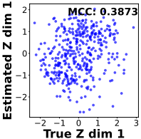
- (a) Scatterplots of Z1 and ˆ Z1.
- (c) Scatterplots of Z2 and ˆ Z1.
- (b) Scatterplots of Z1 and ˆ Z2.
- (d) Scatterplots of Z2 and ˆ Z2.
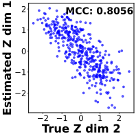
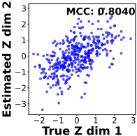
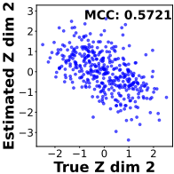
Figure 4: Result on the fifth synthetic dataset. Fig. 4a-4d show the scatterplots between each ground-truth and estimated latent confounder.
| β = 1 | β = 1.5 | β = 3 | β = 4.5 | β = 5 | ||||||
|---|---|---|---|---|---|---|---|---|---|---|
| ϵAT E | ϵITE | ϵAT E | ϵITE | ϵAT E | ϵITE | ϵAT E | ϵITE | ϵAT E | ϵITE | |
| CEVAE | 0.116±0.083 | 0.188±0.081 | 0.324±0.115 | 0.401±0.119 | 3.902±0.740 | 4.162±0.781 | 14.348±3.036 | 15.406±3.493 | 19.403±3.152 | 20.444±3.585 |
| TEDVAE | 0.097±0.039 | 0.205±0.041 | 0.351±0.065 | 0.498±0.068 | 4.356±1.078 | 4.851±1.183 | 16.543±3.757 | 18.589±4.633 | 22.046±3.856 | 24.036±4.571 |
| LTEE | 0.048±0.034 | 0.212±0.071 | 0.296±0.141 | 0.510±0.220 | 4.815±1.269 | 5.726±1.662 | 17.678±7.534 | 20.310±9.404 | 23.980±7.371 | 26.740±9.062 |
| S-Learner | 0.021±0.013 | 0.414±0.091 | 0.096±0.090 | 0.617±0.098 | 2.916±0.854 | 4.186±1.027 | 15.382±7.409 | 19.080±8.705 | 18.842±9.137 | 22.609±10.251 |
| T-Learner | 0.190±0.130 | 0.582±0.193 | 0.209±0.211 | 0.867±0.304 | 5.554±2.733 | 7.687±3.529 | 17.026±6.587 | 21.598±7.321 | 20.068±10.22 | 26.478±9.314 |
| Imputation | 0.792±0.934 | - | 0.928±1.258 | - | 2.480±2.290 | - | 13.156±7.144 | - | 19.518±11.240 | - |
| Weighting | 0.861±0.648 | - | 0.639±0.339 | - | 11.579±6.775 | - | 51.634±13.346 | - | 70.104±11.687 | - |
| Equi-naive | 0.285±0.422 | 0.823±0.353 | 0.247±0.272 | 1.001±0.245 | 2.837±1.377 | 4.297±2.080 | 10.619±14.245 | 14.245±7.583 | 19.314±3.186 | 22.978±3.406 |
| IF-base | 0.619±0.831 | - | 1.707±1.893 | - | 9.385±7.690 | - | 30.562±13.998 | - | 32.723±12.970 | - |
| ICEVAE | 0.038±0.031 | 0.069±0.032 | 0.182±0.086 | 0.217±0.085 | 2.402±0.436 | 3.173±0.418 | 9.897±2.685 | 11.395±2.841 | 14.960±3.363 | 16.467±3.935 |
Does our model perform well on datasets that follow different existing assumptions?
We conduct experiments by comparing our method with baselines on three different synthetic datasets that follow different data generation processes. The results are shown in Table 1. Overall, on all three datasets, our method achieves almost the best performance, revealing the generalizability of our method under different assumptions. In detail, on the Synthetic 1 dataset, our method achieves the lowest ITE and ATE estimation error and std, indicating the effectiveness of our method. As for the results of the Synthetic 2 dataset, compared with baselines, our method achieves comparable performance. Note that the Imputation and Weighting methods perform much better on the Synthetic 2 dataset than the Synthetic 1 dataset since the Synthetic 2 dataset is designed following the latent unconfoundedness assumption. Similarly, as for the results of the Synthetic 3 dataset that is generated following the additive equi-confounding bias assumption, Equi-naive can achieve the lowest error in terms of ATE estimation. On this dataset, our method also achieves comparable performance, especially in terms of ITE estimation. Hence, we conclude that our model can perform well on datasets that follow different existing assumptions.
Does our model outperform baselines on real-world datasets?
In Table 3, we evaluate the performance of our model on complex real-world data by comparing each method using two semi-synthetic datasets. The main observations are as follows. Overall, our method achieves the best performance regarding ITE estimation and comparable performance regarding ATE estimation, indicating the effectiveness of our method. Specifically, compared with the VAE-based method, our method performs better, which indicates that the experimental data does help recover latent confounders. Compared with the Imputation and Weighting methods, our method strongly outperforms them, since the unsuitable latent unconfoundedness assumption is made by their methods. In conclusion, we find that our method ICEVAE can outperform baselines on real-world datasets.
Is our method robust to different strengths of latent confounding?
In table 2, we compare our model with baselines on the fourth synthetic dataset with different strengths of confounding bias controlled by β. The main observations are as follows. With the strengths of latent confounding increasing, i.e., β from 1 to 5, all methods perform worse, which is reasonable since a large confounding bias will lead to a significant imbalance of distribution between treated and control groups. When the latent confounding is small, traditional methods yield a comparable performance, since the unconfoundedness assumption almost holds. When the latent confounding is large enough, only our method yields accurate estimations in terms of ATE and ITE, which indicates that our method is robust to the latent confounding. It is because our method can correctly recover the latent confounders Z, and it also reveals the necessity of recovering latent confounders.
| IHDP | TWINS | |||
|---|---|---|---|---|
| ϵAT E | ϵITE | ϵAT E | ϵITE | |
| CEVAE | 0.004±0.003 | 0.183±0.054 | 0.641±0.521 | 16.818±11.867 |
| TEDVAE | 0.011±0.019 | 0.188±0.032 | 0.824±1.108 | 16.657±11.978 |
| LTEE | 0.015±0.014 | 0.668±0.132 | 1.994±2.470 | 15.667±14.297 |
| T-Leaner | 0.061±0.051 | 1.060±0.214 | 4.665±5.505 | 5.191±5.581 |
| S-Leaner | 0.020±0.018 | 0.969±0.354 | 2.536±4.101 | 12.288±4.779 |
| Imputaion | 0.713±0.478 | - | 46.092±43.729 | - |
| Weighting | 0.664±0.959 | - | 6.597±10.859 | - |
| ICEVAE | 0.016±0.027 | 0.178±0.060 | 0.204±0.229 | 3.665±2.246 |
7 Conclusion
In this paper, we provide a practical solution to estimate the long-term individual causal effects in the presence of latent confounders via identifiable representation learning. Our proposed method takes advantage of the natural heterogeneity of data, e.g., data from multiple cities, to identify latent confounders and further estimate the long-term individual effect, which not only helps us avoid the idealized assumptions of the existing methods, but also renders our approach with theoretical guarantees of identifiability. Extensive experimental results verify the correctness of our theory and the effectiveness of our estimator.
Acknowledgments
This research was supported in part by National Science and Technology Major Project (2021ZD0111501), National Science Fund for Excellent Young Scholars (62122022), Natural Science Foundation of China (U24A20233, 62206064, 62206061, 62476163, 62406078), Guangdong Basic and Applied Basic Research Foundation (2023B1515120020), and CCF-DiDi GAIA Collaborative Research Funds (CCF-DiDi GAIA 202311).
@inproceedings{ijcai2025p533,
  title     = {Long-Term Individual Causal Effect Estimation via Identifiable Latent Representation Learning},
  author    = {Cai, Ruichu and Wan, Junjie and Chen, Weilin and Yang, Zeqin and Li, Zijian and Zhen, Peng and Guo, Jiecheng},
  booktitle = {Proceedings of the Thirty-Fourth International Joint Conference on
               Artificial Intelligence, {IJCAI-25}},
  publisher = {International Joint Conferences on Artificial Intelligence Organization},
  editor    = {James Kwok},
  pages     = {4788--4796},
  year      = {2025},
  month     = {8},
  note      = {Main Track},
  doi       = {10.24963/ijcai.2025/533},
  url       = {https://doi.org/10.24963/ijcai.2025/533},
}
TY - CPAPER TI - Long-Term Individual Causal Effect Estimation via Identifiable Latent Representation Learning AU - Cai, Ruichu AU - Wan, Junjie AU - Chen, Weilin AU - Yang, Zeqin AU - Li, Zijian AU - Zhen, Peng AU - Guo, Jiecheng T2 - Proceedings of the Thirty-Fourth International Joint Conference on Artificial Intelligence, IJCAI-25 PB - International Joint Conferences on Artificial Intelligence Organization PY - 2025 SP - 4788 EP - 4796 DO - 10.24963/ijcai.2025/533 UR - https://doi.org/10.24963/ijcai.2025/533 ER -Copied
Machine-readable versions of this paper, for tools and AI agents:





