
Causal View of Time Series Imputation: Some Identification Results on Missing Mechanism
Proceedings of the Thirty-Fourth International Joint Conference on Artificial Intelligence. Main Track. Pages 4779-4787.
https://doi.org/10.24963/ijcai.2025/532
Keywords
- Machine Learning: ML: Time series and data streams
Abstract
Time series imputation is one of the most challenging problems and has broad applications in various fields like health care and the Internet of Things. Existing methods mainly aim to model the temporally latent dependencies and the generation process from the observed time series data. In real-world scenarios, different types of missing mechanisms, like MAR (Missing At Random) and MNAR (Missing Not At Random), can occur in time series data. However, existing methods often overlook the difference among the aforementioned missing mechanisms and use a single model for time series imputation, which can easily lead to misleading results due to mechanism mismatching. In this paper, we propose a framework for the time series imputation problem by exploring Different Missing Mechanisms (DMM in short) and tailoring solutions accordingly. Specifically, we first analyze the data generation processes with temporal latent states and missing cause variables for different mechanisms. Sequentially, we model these generation processes via variational inference and estimate prior distributions of latent variables via a normalizing flow-based neural architecture. Furthermore, we establish identifiability results under the nonlinear independent component analysis framework to show that latent variables are identifiable. Experimental results show that our method surpasses existing time series imputation techniques across various datasets with different missing mechanisms, demonstrating its effectiveness in real-world applications.
- [Acuna and Rodriguez, 2004] Edgar Acuna and Caroline Rodriguez. The treatment of missing values and its ef- fect on classifier accuracy. In Classification, Clustering, and Data Mining Applications: Proceedings of the Meet- ing of the International Federation of Classification So- cieties (IFCS), Illinois Institute of Technology, Chicago, 15-18 July 2004, pages 639-647. Springer, 2004.
- [Alcaraz and Strodthoff, 2022] Juan Miguel Lopez Alcaraz and Nils Strodthoff. Diffusion-based time series impu- tation and forecasting with structured state space models. arXiv preprint arXiv:2208.09399, 2022.
- [Cai et al., 2025a] Ruichu Cai, Haiqin Huang, Zhifan Jiang, Zijian Li, Changze Zhou, Yuequn Liu, Yuming Liu, and Zhifeng Hao. Disentangling long-short term state under unknown interventions for online time series forecasting. In Proceedings of the AAAI Conference on Artificial Intel- ligence, volume 39, pages 15641-15649, 2025.
- [Cai et al., 2025b] Ruichu Cai, Zhifan Jiang, Kaitao Zheng, Zijian Li, Weilin Chen, Xuexin Chen, Yifan Shen, Guangyi Chen, Zhifeng Hao, and Kun Zhang. Learning disentangled representation for multi-modal time-series sensing signals. In Proceedings of the ACM on Web Con- ference 2025, pages 3247-3266, 2025.
- [Cai et al., 2025c] Ruichu Cai, Junjie Wan, Weilin Chen, Ze- qin Yang, Zijian Li, Peng Zhen, and Jiecheng Guo. Long- term individual causal effect estimation via identifiable la- tent representation learning. 2025.
- [Cao et al., 2018] Wei Cao, Dong Wang, Jian Li, Hao Zhou, Lei Li, and Yitan Li. Brits: Bidirectional recurrent im- putation for time series. Advances in neural information processing systems, 31, 2018.
- [Che et al., 2018] Zhengping Che, Sanjay Purushotham, Kyunghyun Cho, David Sontag, and Yan Liu. Recurrent neural networks for multivariate time series with missing values. Scientific reports, 8(1):6085, 2018.
- [Chen et al., 2023] Yu Chen, Wei Deng, Shikai Fang, Feng- pei Li, Nicole Tianjiao Yang, Yikai Zhang, Kashif Rasul, Shandian Zhe, Anderson Schneider, and Yuriy Nevmy- vaka. Provably convergent schrödinger bridge with appli- cations to probabilistic time series imputation. In Inter- national Conference on Machine Learning, pages 4485- 4513. PMLR, 2023.
- [Choi and Lee, 2023] MinGyu Choi and Changhee Lee. Conditional information bottleneck approach for time se- ries imputation. In The Twelfth International Conference on Learning Representations, 2023.
- [Du et al., 2023] Wenjie Du, David Côté, and Yan Liu. Saits: Self-attention-based imputation for time series. Expert Systems with Applications, 219:119619, 2023.
- [Fang et al., 2023] Shikai Fang, Qingsong Wen, Shandian Zhe, and Liang Sun. Bayotide: Bayesian online multivari- ate time series imputation with functional decomposition. arXiv preprint arXiv:2308.14906, 2023.
- [Fortuin et al., 2020] Vincent Fortuin, Dmitry Baranchuk, Gunnar Rätsch, and Stephan Mandt. Gp-vae: Deep proba- bilistic time series imputation. In International conference on artificial intelligence and statistics, pages 1651-1661.
- PMLR, 2020.
- [Jiang et al., 2023] Jiawei Jiang, Chengkai Han, Wayne Xin Zhao, and Jingyuan Wang. Pdformer: Propagation delay- aware dynamic long-range transformer for traffic flow pre- diction. In Proceedings of the AAAI conference on artifi- cial intelligence, volume 37, pages 4365-4373, 2023.
- [Kong et al., 2022] Lingjing Kong, Shaoan Xie, Weiran Yao, Yujia Zheng, Guangyi Chen, Petar Stojanov, Victor Akin- wande, and Kun Zhang. Partial disentanglement for do- main adaptation. In International conference on machine learning, pages 11455-11472. PMLR, 2022.
- [Lai et al., 2018] Guokun Lai, Wei-Cheng Chang, Yiming Yang, and Hanxiao Liu. Modeling long-and short-term temporal patterns with deep neural networks. In The 41st international ACM SIGIR conference on research & devel- opment in information retrieval, pages 95-104, 2018.
- [Li et al., 2024a] Zijian Li, Ruichu Cai, Guangyi Chen, Boyang Sun, Zhifeng Hao, and Kun Zhang. Subspace identification for multi-source domain adaptation. Ad- vances in Neural Information Processing Systems, 36, 2024.
- [Li et al., 2024b] Zijian Li, Ruichu Cai, Zhenhui Yang, Haiqin Huang, Guangyi Chen, Yifan Shen, Zhengming Chen, Xiangchen Song, and Kun Zhang. When and how: Learning identifiable latent states for nonstationary time series forecasting. arXiv preprint arXiv:2402.12767, 2024.
- [Li et al., 2025] Zijian Li, Yifan Shen, Kaitao Zheng, Ruichu Cai, Xiangchen Song, Mingming Gong, Guangyi Chen, and Kun Zhang. On the identification of temporal causal representation with instantaneous dependence. In The Thirteenth International Conference on Learning Repre- sentations, 2025.
- [Liu et al., 2023] Yong Liu, Tengge Hu, Haoran Zhang, Haixu Wu, Shiyu Wang, Lintao Ma, and Mingsheng Long. itransformer: Inverted transformers are effective for time series forecasting. arXiv preprint arXiv:2310.06625, 2023.
- [Locatello et al., 2019] Francesco Locatello, Stefan Bauer, Mario Lucic, Gunnar Raetsch, Sylvain Gelly, Bernhard Schölkopf, and Olivier Bachem. Challenging common assumptions in the unsupervised learning of disentangled representations. In international conference on machine learning, pages 4114-4124. PMLR, 2019.
- [Luo et al., 2018] Yonghong Luo, Xiangrui Cai, Ying Zhang, Jun Xu, et al. Multivariate time series imputation with generative adversarial networks. Advances in neural information processing systems, 31, 2018.
- [Miao et al., 2021] Xiaoye Miao, Yangyang Wu, Jun Wang, Yunjun Gao, Xudong Mao, and Jianwei Yin. Generative semi-supervised learning for multivariate time series im- putation. In Proceedings of the AAAI conference on artifi- cial intelligence, volume 35, pages 8983-8991, 2021.
- [Mohan et al., 2013] Karthika Mohan, Judea Pearl, and Jin Tian. Graphical models for inference with missing data. Advances in neural information processing systems, 26, 2013.
- [Nie et al., 2023] Tong Nie, Guoyang Qin, Wei Ma, Yuewen Mei, and Jian Sun. Imputeformer: Low rankness-induced transformers for generalizable spatiotemporal imputation. arXiv: 2312.01728, 2023.
- [Rubin, 1976] Donald B Rubin. Inference and missing data. Biometrika, 63(3):581-592, 1976.
- [Tang and Matteson, 2021] Binh Tang and David S Matte- son. Probabilistic transformer for time series analy- sis. Advances in Neural Information Processing Systems, 34:23592-23608, 2021.
- [Tashiro et al., 2021] Yusuke Tashiro, Jiaming Song, Yang Song, and Stefano Ermon. Csdi: Conditional score- based diffusion models for probabilistic time series impu- tation. Advances in Neural Information Processing Sys- tems, 34:24804-24816, 2021.
- [Van Buuren and Groothuis-Oudshoorn, 2011] Stef Van Bu- uren and Karin Groothuis-Oudshoorn. mice: Multivariate imputation by chained equations in r. Journal of statistical software, 45:1-67, 2011.
- [Wu et al., 2022] Haixu Wu, Tengge Hu, Yong Liu, Hang Zhou, Jianmin Wang, and Mingsheng Long. Timesnet: Temporal 2d-variation modeling for general time series analysis. arXiv preprint arXiv:2210.02186, 2022.
- [Wu et al., 2023] Haixu Wu, Hang Zhou, Mingsheng Long, and Jianmin Wang. Interpretable weather forecasting for worldwide stations with a unified deep model. Nature Ma- chine Intelligence, 5(6):602-611, 2023.
- [Yao et al., 2021] Weiran Yao, Yuewen Sun, Alex Ho, Changyin Sun, and Kun Zhang. Learning temporally causal latent processes from general temporal data. arXiv preprint arXiv:2110.05428, 2021.
- [Yao et al., 2022] Weiran Yao, Guangyi Chen, and Kun Zhang. Temporally disentangled representation learn- ing. Advances in Neural Information Processing Systems, 35:26492-26503, 2022.
- [Zhang et al., 2021] Ying Zhang, Baohang Zhou, Xiangrui Cai, Wenya Guo, Xiaoke Ding, and Xiaojie Yuan. Miss- ing value imputation in multivariate time series with end- to-end generative adversarial networks. Information Sci- ences, 551:67-82, 2021.
- [Zhou et al., 2021] Haoyi Zhou, Shanghang Zhang, Jieqi Peng, Shuai Zhang, Jianxin Li, Hui Xiong, and Wan- cai Zhang. Informer: Beyond efficient transformer for long sequence time-series forecasting. In Proceedings of the AAAI conference on artificial intelligence, volume 35, pages 11106-11115, 2021.
References were extracted automatically from the PDF and may contain errors.
Full text extracted automatically from the PDF; figures, tables and equations may differ. The PDF is the version of record.
1 Introduction
While data-driven deep models have achieved significant performance on time series analysis 1 [Tang and Matteson, 2021;
∗Corresponding author.
1 The extended version: https://arxiv.org/abs/2505.07180.
Wu et al., 2022] and massive applications, like traffic [Jiang et al., 2023; Cai et al., 2025a], weather [Wu et al., 2023], and the Internet of Things [Cai et al., 2025b], their prosperity usually requires complete data. However, the missing values of time series led by sensor failures hinder the deployment of existing algorithms to real-world scenarios. To address this challenge, time series imputation [Nie et al., 2023; Fang et al., 2023] is proposed. The primary goal of time series imputation is to leverage the observed data and the missing indicators to identify the distribution of time series data.
To identify the distribution from the time series data[Li et al., 2025], different approaches have been proposed to identify the distribution from the time series data with missing values[Li et al., 2024b]. Previously, researchers used statistical tools [Acuna and Rodriguez, 2004; Van Buuren and Groothuis-Oudshoorn, 2011] to address the time series imputation. Recent methods based on deep neural networks can be categorized into predictive and generative methods. For example, the predictive models harness different neural architectures like recursive neural networks [Cao et al., 2018; Che et al., 2018], convolution neural networks [Wu et al., 2022], and Transformer [Nie et al., 2023; Liu et al., 2023] to model the inherent dependencies of among variables. Additionally, the generative methods use varied deep generative models like variational autoencoders (VAE) [Choi and Lee, 2023; Fortuin et al., 2020; Cai et al., 2025c], generative adversarial networks (GANs) [Luo et al., 2018; Zhang et al., 2021], and diffusion models [Alcaraz and Strodthoff, 2022; Tashiro et al., 2021; Chen et al., 2023] to model the distribution of complete time series data. In summary, these methods model the temporal latent process and generation from latent to observed variables for missing value imputation. Please refer to Appendix A for related work on time series imputation and identification of the temporal latent process.
In practical applications, time series data can be affected by various types of missing data mechanisms, such as MCAR (Missing Completely At Random), MAR (Missing At Random), and MNAR (Missing Not At Random). While current methods have achieved success in time series imputation, they often employ a single model that does not account for the differences between these mechanisms. Given an example in healthcare that follows the MNAR mechanisms, patients who experience worsening conditions may not return for scheduled follow-ups, resulting in missing data for the later stages of the treatment. In this case, if a model uses a mismatched missing mechanism like MCAR and ignores the dependency between the missing format and the observed values, it is hard for it to achieve an accurate imputation performance. Therefore, it is essential for time series imputation to model the time series data according to different missing mechanisms.
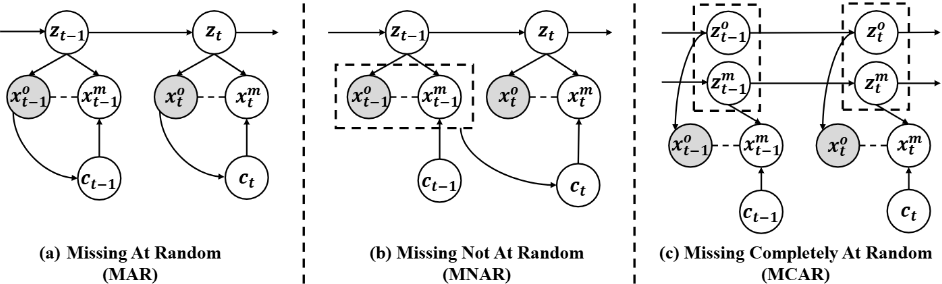
To better exploit the missing mechanisms, we explore Different Missing Mechanisms and propose the corresponding methods, forming a general framework named DMM. We first analyze the data generation processes of time series data under different missing mechanisms, including MAR, MNAR, and MCAR. [Locatello et al., 2019] find that the MCAR mechanism is not identifiable and is rare in real-world scenarios. Based on the aforementioned data generation processes, we employ variational inference to model how missing data are generated and the normalizing flow-based neural architectures to enforce the identification of latent variables. Moreover, we analyze the identification results for different missing mechanisms, in which the temporal latent variables and latent missing causes can be identified in the case of MAR and MNAR. Our approach is validated through massive semisynthetic datasets on all the missing mechanisms, the experimental results show that our DMM method outperforms the state-of-the-art baselines. Please refer to Appendix D for more details on the missing mechanism.
2 Preliminaries
In this paper, we focus on the time series imputation problem in the presence of various types of missing mechanisms. We first formalize the generation process for the time series imputation problem, and then introduce a graphical model (termed imputation m-graphs) to represent it.
Data-generating process. We first let the time series data X = {x1, x2, · · · , xT}, xt ∈ Rn be generated from latent variables zt ∈ Z ⊆ Rn by an invertible and nonlinear mixing function g as shown in Equation (1):
Moreover, the i-th dimension latent variable zt,i is timedelayed and causally related to the historical latent variables zt-τ with the time lag τ via a nonparametric function fi, which is shown as in Equation (2).
where Pa(zt,i) denotes the set of latent variables that directly cause zt,i and ϵt,i denotes the temporally and spatially independent noise extracted from a distribution Pϵt,i . Here, we provide a medical example to explain this data generation process. First, we let xt be the measurable index, like body temperature or blood pressure. And then zt can be considered as the virus concentration, which is hard to measure.
Graphical Notation. To describe the time series data with missing values, given an entire time series data xt, we further partition the time series data into the observed variables xot and missing variables xmt , such that xt = xot ∪xmt . To model the generation process xt, we use the missing graph with imputation problems (abbreviated as imputation m-graphs) such that xt can be represented by a causal graph, where the gray nodes represent observed variables, and the white nodes represent unobserved variables. Note that this graph differs from the m-graph [Mohan et al., 2013], where, in the imputation m-graph, the missing variable is determined by its cause variables. Since the direct causal relationships between observed and missing variables are unknown (e.g., the edge between xot and xmt exist or not), we use dashed lines to represent these uncertain connections. Based on the imputation m-graph, one can easily distinguish different missing mechanisms for the imputation problem, leading to more general identifiability results (See the identification results section).
Objectives. In the context of time series imputation, we assume that the existence of a training set {Xo i ,Xm i }Mi=1 with the size of M. While in the I.I.D test set, we can only access {Xo i }Ti=1 with the size of T, our goal is to use the training dataset to obtain a model, such that it can identify the distribution P(Xo ,Xm) of test data.
As mentioned above, existing methods may suffer from mechanism mismatching problems since they usually use one model to cover all the missing mechanisms, making it hard to identify the distribution P(Xo ,Xm). In general, all missing data problems fall into one of the following mechanisms [Rubin, 1976]: missing completely at random (MCAR), missing at random (MAR), and missing not at random (MNAR). Fortunately, with the imputation m-graph, these missing mechanisms can be precisely categorized by incorporating the missing cause variables ct, which are introduced as follows.
2.1 Missing At Random
When data are Missing At Random (MAR), the missingness is related to known variables but not to the values that are missing. Specifically, the missing cause variables are influenced by the observed variables, and they further lead to the missingness. Suppose the time series data are generated by the latent process shown in Eq. (1) and Eq. (2), the MAR missingness can be further represented by Figure 1(a), where the missing cause variables ct (ct → xmt ) are influenced by the observed variable xot (i.e., xot → ct). The dashed edge in Figure 1(a) between xmt and xot indicates that we allow a direct causal relationship between them.
By combining the generating process and Figure 1 (a), the joint distribution in MAR can be formalized as:
where z1:T := {z1, · · · , zT} and c1:T := {c1, · · · , cT}. In this case, we can identify the joint distribution by modeling 1) generative model P (xm1:T |c1:T , z1:T , xo1:T ) of missing values; 2) the conditional distributions of missing cause and latent variables, i.e., P (c1:T |xo1:T ) and P (z1:T |xo1:T ).
Establishing the joint distribution for MAR allows us to perform accurate variational inference to recover the distribution p(zt) and p(ct), and identify P (Xo , Xm) accordingly (see implementation section).
2.2 Missing Not At Random
When data are Missing Not At Random (MNAR), the missingness depends on unobserved data. Specifically, the missing causes are influenced by the historical missing variables, and they further lead to the current missingness. Suppose the time series data are generated by the latent process shown in Eq. (1) and Eq. (2), the MNAR missingness can be further described by Figure 1(b), where the missing causes ct (ct → xmt ) are influenced by historical missing variables xot-1 and xmt-1 , i.e., xot-1 → ct&xmt-1 → ct. The dashed box in Figure 1(b) means that both xot-1 and xmt-1 are causes of ct. Similarly, based on the corresponding imputation mgraph, the joint distribution can be formalized as:
where z1:T := {z1, · · · , zT} and c1:T := {c1, · · · , cT}. In this case, we can identify the joint distribution by modeling 1) generative model P(xmt |ct, zt, xot ) of missing values; 2) the conditional distributions of missing cause and latent variables, i.e., P(ct|xt-1) and P(zt|xot ).
2.3 Missing Completely At Random
When data are Missing Completely At Random (MCAR), however, it is impossible to reconstruct the latent process and recover p(xo1:T , xm1:T ), since the missingness is independent of all other variables, as shown in Figure 1(c).
| Dataset | Ratio | DMM-MAR | DMM-MNAR | TimeCIB | ImputeFormer | TimesNet | SAITS | GPVAE | CSDI | BRITS MAE | SSGAN | ||||||||||
|---|---|---|---|---|---|---|---|---|---|---|---|---|---|---|---|---|---|---|---|---|---|
| MSE | MAE | MSE | MAE | MSE | MAE | MSE | MAE | MSE | MAE | MSE | MAE | MSE | MAE | MSE | MAE | MSE | MSE | MAE | |||
| 0.2 | 0.099 | 0.212 | 0.118 | 0.232 | 0.285 | 0.405 | 0.666 | 0.510 | 0.139 | 0.241 | 0.252 | 0.312 | 0.213 | 0.339 | 0.334 | 0.327 | 0.115 | 0.239 | 0.152 | 0.279 | |
| ETTh1 0.4 | 0.165 | 0.259 | 0.184 | 0.297 | 0.389 | 0.471 | 0.705 | 0.579 | 0.207 | 0.294 | 0.185 | 0.286 | 0.280 | 0.407 | 0.523 | 0.438 | 0.175 | 0.277 | 0.172 | 0.280 | |
| 0.6 | 0.217 | 0.302 | 0.440 | 0.436 | 0.497 | 0.519 | 0.766 | 0.608 | 0.374 | 0.419 | 0.401 | 0.420 | 0.585 | 0.572 | 0.732 | 0.554 | 0.265 | 0.368 | 0.256 | 0.345 | |
| 0.2 | 0.113 | 0.228 | 0.153 | 0.270 | 0.471 | 0.319 | 0.343 | 0.420 | 0.150 | 0.242 | 0.143 | 0.277 | 0.411 | 0.487 | 0.306 | 0.350 | 0.329 | 0.415 | 0.371 | 0.470 | |
| ETTh2 0.4 | 0.214 | 0.339 | 0.233 | 0.347 | 0.543 | 0.487 | 0.542 | 0.551 | 0.386 | 0.434 | 0.672 | 0.591 | 0.463 | 0.521 | 0.567 | 0.484 | 0.444 | 0.486 | 0.747 | 0.692 | |
| 0.6 | 0.204 | 0.313 | 0.206 | 0.317 | 0.767 | 0.601 | 0.548 | 0.558 | 0.260 | 0.322 | 0.313 | 0.409 | 0.660 | 0.634 | 1.100 | 0.688 | 0.695 | 0.641 | 1.547 | 0.965 | |
| 0.2 | 0.029 | 0.112 | 0.040 | 0.136 | 0.067 | 0.189 | 0.573 | 0.477 | 0.080 | 0.178 | 0.030 | 0.114 | 0.077 | 0.198 | 0.038 | 0.119 | 0.038 | 0.126 | 0.059 | 0.169 | |
| ETTm1 0.4 | 0.039 | 0.129 | 0.061 | 0.165 | 0.099 | 0.229 | 0.585 | 0.488 | 0.127 | 0.221 | 0.041 | 0.134 | 0.109 | 0.237 | 0.049 | 0.132 | 0.046 | 0.137 | 0.078 | 0.198 | |
| 0.6 | 0.060 | 0.163 | 0.084 | 0.202 | 0.183 | 0.324 | 0.574 | 0.496 | 0.211 | 0.282 | 0.062 | 0.163 | 0.166 | 0.293 | 0.077 | 0.171 | 0.062 | 0.163 | 0.078 | 0.191 | |
| 0.2 | 0.041 | 0.130 | 0.042 | 0.135 | 0.338 | 0.447 | 0.130 | 0.267 | 0.063 | 0.162 | 0.060 | 0.171 | 0.400 | 0.465 | 0.061 | 0.105 | 0.126 | 0.248 | 0.221 | 0.374 | |
| ETTm2 0.4 | 0.044 | 0.138 | 0.055 | 0.155 | 0.444 | 0.506 | 0.177 | 0.303 | 0.085 | 0.187 | 0.070 | 0.184 | 0.401 | 0.479 | 0.141 | 0.149 | 0.166 | 0.288 | 0.129 | 0.261 | |
| 0.6 | 0.053 | 0.157 | 0.075 | 0.184 | 0.715 | 0.626 | 0.161 | 0.290 | 0.128 | 0.228 | 0.108 | 0.229 | 0.481 | 0.516 | 0.335 | 0.242 | 0.298 | 0.395 | 0.211 | 0.336 | |
| 0.2 | 0.003 | 0.038 | 0.009 | 0.051 | 0.314 | 0.281 | 0.178 | 0.283 | 0.013 | 0.063 | 0.085 | 0.231 | 0.711 | 0.712 | 0.017 | 0.076 | 0.319 | 0.493 | 0.666 | 0.711 | |
| Exchange 0.4 | 0.007 | 0.049 | 0.023 | 0.106 | 0.388 | 0.326 | 0.158 | 0.273 | 0.017 | 0.081 | 0.193 | 0.350 | 0.783 | 0.751 | 0.018 | 0.078 | 0.431 | 0.580 | 0.820 | 0.773 | |
| 0.6 | 0.008 | 0.058 0.050 | 0.030 0.049 | 0.121 0.084 | 0.445 | 0.372 | 0.201 | 0.296 0.153 | 0.024 | 0.101 0.077 | 0.224 0.040 | 0.382 0.078 | 0.834 0.055 | 0.771 0.128 | 0.055 0.069 | 0.143 0.057 | 0.669 0.034 | 0.707 0.059 | 1.235 0.035 | 0.961 | |
| 0.4 | 0.035 | 0.059 | 0.061 | 0.104 | 0.062 | 0.128 | 0.110 | 0.165 | 0.050 | 0.103 | 0.047 | 0.075 | 0.047 | 0.069 | 0.077 | ||||||
| Weather 0.2 | 0.029 | 0.049 | 0.113 | 0.099 | 0.038 | 0.085 | 0.073 | 0.141 | 0.061 | 0.042 | 0.089 | ||||||||||
| 0.6 | 0.040 | 0.070 | 0.080 | 0.132 | 0.082 | 0.152 | 0.110 | 0.167 | 0.061 | 0.119 | 0.058 | 0.090 | 0.082 | 0.160 | 0.074 | 0.053 | 0.072 | 0.058 | 0.053 | 0.111 | |
In this case, distribution p(xo1:T , xm1:T ) = ∫zo1:T ,zm1:T ,c1:T p(xo1:T |zo1:T )p(xm1:T |zm1:T , c1:T )p(zo1:T , zm1:T , c1:T )dzm1:T dzo1:T dc1:T are not identifiable since it is hard to identify p(zo1:T , zm1:T , c1:T ) without further auxiliary variables [Locatello et al., 2019].
In real-world scenarios, this case is rare since complex relationships exist among latent variables, making the observed and missing variables are not independent. Since the MCAR mechanism is rare in real-world scenarios, we mainly investigate the time series imputation problem under the MAR and MNAR scenarios.
3 Implementation of DMMFramework
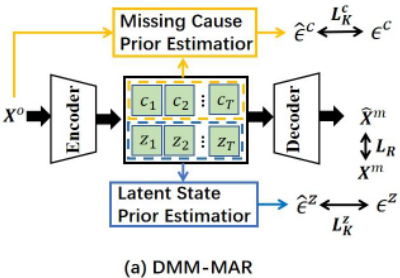
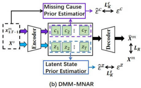
Based on these data generation processes, we introduce the DMM framework as shown in Figure 2, which models the data generation process of MAR and MNAR mechanisms. Specifically, the DMM framework contains two models, which we name for MAR and MNAR mechanisms DMMMAR and DMM-MNAR, respectively. Please refer to Appendix F for implementation details.
3.1 DMM-MARmodel
The DMM-MAR model is shown in Figure 2(a), which is built on a variational inference neural architecture with prior estimators for latent states and missing cause variables.
Sequential Variational Backbone architecture for DMMMAR. We effectively leverage the variational autoencoder to model the time series data. Specifically, for the data generation process of MAR, we have the following approach:
where DKL denotes the KL divergence. Specifically, q(z1:T |xo1:T ) and q(c1:T |xo1:T ) denote the encoders for the latent states zt and missing cause variables ct, which are used to approximate the prior distribution. Technologically, these encoders can be formalized as follows:
where ϕAz and ϕAc 2 denote the latent states encoder and the missing cause encoder, respectively. Moreover, p(xm1:T |z1:T , c1:T ) denote the decoder for missing value prediction, which is formalized as follows:
where FA denotes the predictor and it is implemented by Multi-layer Perceptron networks (MLPs).
3.2 Prior Estimator for Temporal Latent States and Missing Cause Variables
To model the prior distributions of temporal latent states and missing cause variables, we propose the latent state prior estimator and the missing cause prior estimator, respectively.
As for the latent state prior estimator, we first let {rA i } be a set of learned inverse transition functions that take the estimated latent variables and output the noise term, i.e., ˆ ϵzt,i = rA i (ˆ zt,i, ˆzt-1) and each rA i is modeled with MLPs. Then we devise a transformation ψA z := {ˆzt-1, ˆzt} → {ˆzt-1, ˆ ϵzt },
denotes a matrix. By applying the change of variables formula, we have the following equation:
Since we explicitly assume that the noise term in Equation (2) is entirely independent with zt-1, we enforce the independence of the estimated noise ˆ ϵzt and we have:
Therefore, the latent state prior can be estimated as follows: ln p(ˆz1:t) = ln p(ˆz1)
2 We use the superscript symbol to denote estimated variables
| Dataset | Ratio | DMM-MAR | DMM-MNAR | TimeCIB | ImputeFormer | TimesNet | SAITS | GPVAE | CSDI | BRITS | SSGAN | ||||||||||
|---|---|---|---|---|---|---|---|---|---|---|---|---|---|---|---|---|---|---|---|---|---|
| MSE | MAE | MSE | MAE | MSE | MAE | MSE | MAE | MSE | MAE | MSE | MAE | MSE | MAE | MSE | MAE | MSE | MAE | MSE | MAE | ||
| 0.2 | 0.138 | 0.240 | 0.108 | 0.230 | 0.327 | 0.475 | 0.651 | 0.503 | 0.149 | 0.248 | 0.165 | 0.271 | 0.256 | 0.375 | 0.326 | 0.324 | 0.125 | 0.248 | 0.149 | 0.281 | |
| ETTh1 0.4 | 0.238 | 0.329 | 0.171 | 0.280 | 0.392 | 0.492 | 0.691 | 0.530 | 0.220 | 0.306 | 0.265 | 0.330 | 0.362 | 0.442 | 0.497 | 0.424 | 0.177 | 0.294 | 0.172 | 0.301 | |
| 0.6 | 0.323 | 0.384 | 0.262 | 0.358 | 0.484 | 0.517 | 0.689 | 0.538 | 0.309 | 0.373 | 0.308 | 0.363 | 0.405 | 0.467 | 0.659 | 0.521 | 0.297 | 0.388 | 0.271 | 0.377 | |
| 0.2 | 0.088 | 0.197 | 0.078 | 0.187 | 0.501 | 0.416 | 0.172 | 0.348 | 0.127 | 0.230 | 0.143 | 0.273 | 0.389 | 0.486 | 0.229 | 0.309 | 0.211 | 0.334 | 0.306 | 0.421 | |
| ETTh2 0.4 | 0.099 | 0.216 | 0.089 | 0.200 | 0.563 | 0.482 | 0.299 | 0.387 | 0.187 | 0.273 | 0.218 | 0.340 | 0.572 | 0.573 | 0.516 | 0.472 | 0.293 | 0.402 | 0.653 | 0.644 | |
| 0.6 | 0.178 | 0.268 | 0.133 | 0.255 | 0.647 | 0.569 | 0.450 | 0.471 | 0.325 | 0.353 | 0.293 | 0.396 | 0.831 | 0.704 | 0.946 | 0.646 | 0.547 | 0.580 | 0.334 | 0.423 | |
| 0.2 | 0.038 | 0.131 | 0.025 | 0.104 | 0.079 | 0.206 | 0.608 | 0.481 | 0.082 | 0.179 | 0.028 | 0.110 | 0.080 | 0.204 | 0.032 0.110 | 0.031 | 0.113 | 0.059 | 0.166 | ||
| ETTm1 0.4 | 0.053 | 0.157 | 0.039 | 0.133 | 0.104 | 0.242 | 0.576 | 0.480 | 0.128 | 0.222 | 0.042 | 0.133 | 0.104 | 0.230 | 0.049 | 0.134 | 0.041 | 0.139 | 0.074 | 0.192 | |
| 0.6 | 0.075 | 0.192 | 0.061 | 0.168 | 0.146 | 0.289 | 0.591 | 0.501 | 0.208 | 0.281 | 0.066 | 0.171 | 0.156 | 0.287 | 0.088 | 0.179 | 0.073 | 0.179 | 0.070 | 0.182 | |
| 0.2 | 0.047 | 0.135 | 0.045 | 0.134 | 0.439 | 0.497 | 0.124 | 0.251 | 0.059 | 0.157 | 0.046 | 0.143 | 0.226 | 0.351 | 0.059 | 0.189 | 0.127 | 0.254 | 0.164 | 0.310 | |
| ETTm2 0.4 | 0.052 | 0.148 | 0.049 | 0.146 | 0.569 | 0.579 | 0.151 | 0.274 | 0.115 | 0.213 | 0.076 | 0.194 | 0.413 | 0.489 | 0.061 | 0.194 | 0.159 | 0.277 | 0.085 | 0.193 | |
| 0.6 | 0.072 | 0.174 | 0.066 | 0.174 | 0.647 | 0.782 | 0.142 | 0.271 | 0.158 | 0.243 | 0.090 | 0.206 | 0.500 | 0.523 | 0.096 | 0.254 | 0.221 | 0.324 | 0.159 | 0.280 | |
| 0.2 | 0.007 | 0.052 | 0.004 | 0.044 | 0.526 | 0.471 | 0.150 | 0.262 | 0.014 | 0.070 | 0.117 | 0.274 | 0.749 | 0.741 | 0.016 | 0.076 | 0.461 | 0.574 | 0.586 | 0.651 | |
| Exchange 0.4 | 0.007 | 0.060 | 0.006 | 0.053 | 0.552 | 0.479 | 0.201 | 0.298 | 0.016 | 0.079 | 0.191 | 0.342 | 0.790 | 0.760 | 0.015 | 0.077 | 0.565 | 0.637 | 0.756 | 0.729 | |
| 0.6 0.2 | 0.009 0.054 | 0.063 0.087 | 0.008 0.032 | 0.061 0.052 | 0.574 0.045 | 0.487 | 0.488 0.105 | 0.578 0.148 | 0.024 0.041 | 0.099 0.077 | 0.212 0.041 | 0.370 0.071 | 0.808 0.055 | 0.765 0.116 | 0.041 0.059 | 0.135 0.065 | 0.747 0.037 | 0.750 0.056 | 0.811 0.035 | 0.765 0.073 | |
| 0.4 | 0.041 | 0.069 | 0.038 | 0.062 | 0.061 | 0.126 | 0.104 | 0.157 | 0.054 | 0.093 | 0.050 | 0.076 | 0.073 | 0.057 | 0.067 | ||||||
| Weather | 0.094 | 0.075 | 0.147 | 0.080 | 0.042 | 0.090 | |||||||||||||||
| 0.6 | 0.071 | 0.119 | 0.043 | 0.075 | 0.074 | 0.139 | 0.113 | 0.160 | 0.066 | 0.117 | 0.057 | 0.093 | 0.091 | 0.166 | 0.082 | 0.093 | 0.070 | 0.079 | 0.048 | 0.093 | |
where p(ˆ ϵzi ) follow Gaussian distributions. And another prior p(ˆzt+1:T |ˆz1:t) follows a similar derivation.
As for the missing cause prior estimator, we methodically employ a similar derivation. Then, we specifically designate {sAi } as a set of learned inverse transition functions, which take the observed variables xot and the missing cause ˆct as input, and output the noise term, i.e. ˆ ϵct = sAi (xot , ˆ ct,i).
Leaving sAi be an MLP, we further devise another transformation ψA c := {xot , ˆct} → {xot , ˆ ϵct } with its Jacobian is JψA c = (I 0 ∗ diag ( ∂sAi ∂ˆ ct,i )), where ∗ denotes a matrix. Sim-
ilar to the derivation of latent state prior, we have:
Therefore, the missing cause prior can be estimated by maximizing the following equation, obtained by summing Equation (11) across time steps from 1 to t.
3.3 DMM-MNARmodel
To effectively address the time series imputation model under the MNAR mechanism, we devise the DMM-MNAR model, which is clearly shown in Figure 2(b).
Sequential Variational Backbone architecture for DMMMNAR Similar to the DMM-MARmodel, we employ variational inference to model the data generation process of the MNAR mechanism, and the ELBO is
where DKL denotes the KL divergence. Similar to DMMMNAR, we let q(z1:T |xo1:T ) and q(c1:T |x1:T-1) denote the encoders for the latent states zt and missing cause variables ct. They are formalized as follows:
Moreover, p(x1:T |z1:T , c1:T ) denote the decoder for missing value prediction, which is formalized as follows:
where FB denotes the predictor and it is implemented by Multi-layer Perceptron networks (MLPs).
3.4 Prior Estimator for Temporal Latent States and Missing Cause Variables
Similarly, we also propose the latent state prior estimator and the missing cause prior estimator to model the prior distributions of temporal latent states and missing cause variables.
As for the latent state prior estimator, we first let {rB i } be a set of learned inverse transition functions that take the estimated latent variables and output the noise term, i.e., ˆ εzt,i = rB i (ˆ zt,i, ˆzt-1) and each rB i is modeled with MLPs. Then we devise a transformation ψB z := {ˆzt-1, ˆzt} → {ˆzt-1, ˆ εzt }, and its Jacobian is JψB z = (I 0 ∗ diag ( ∂rB i ∂ˆ zt-1,i )), where ∗
denotes a matrix. By applying the change of variables formula, we have the following equation:
Since we explicitly assume that the noise term in Equation (2) is entirely independent with zt-1, we enforce the independence of the estimated noise ˆ εzt and we have:
Therefore, the latent state prior can be estimated as follows:
where p(ˆ εzi ) follow Gaussian distributions. And another prior p(ˆzt+1:T |ˆz1:t) follows a similar derivation.
As for the missing cause prior estimator, we employ a similar derivation and let {sBi } be a set of learned inverse transition functions, which take the time series data xt-1 and missing cause ˆct as input and output the noise term, i.e. ˆ εct = sBi (xot-1 , ˆxmt-1 , ˆ ct,i).
Leaving sBi be an MLP, we further devise another transformation ψB c := {xot-1 , ˆxmt-1 , ˆct} → {xot-1 , ˆxmt-1 , ˆ εct } with its Jacobian is JψB c = (I 0 ∗ diag ( ∂sBi ∂ˆ ct,i )), where ∗ denotes
a matrix. Similar to latent state prior derivation, we have:
Therefore, the missing cause prior can be estimated by maximizing the following equation:
3.5 Model Summary
The difference between the DMM-MAR and DMM-MNAR is the prior estimator. For DMM-MAR, we use the xot to estimate the prior distribution of ct. For DMM-MNAR, we use the xot-1 and xmt-1 to estimate the prior distribution of ct.
By estimating the prior distribution of latent states and missing causes, we can calculate the KL divergence in Equations (5) and (13). So we can optimize the ELBO to model the data generation processes. The total loss of the proposed two models can be formalized as follows:
where β and γ are hyperparameters.
In real-world scenarios full of complexity, we do not know which type of missing data mechanism applies. However, we can use model selection methods by running two models on the same data and choosing the one that yields better results. We will verify this in the experimental section.
4 Identification Results
In this section, we aim to show that the identifiability for latent state zt and missing causes ct under the MAR and MNAR missing mechanisms, providing a theoretical guarantee for the DMM framework. Specifically, we say zt is 'identifiable' if, for each ground-truth changing latent variables zt, there exists a corresponding estimated component ˆzt and an invertible function hz : Rn → Rn , such that zt = hz (ˆzt). The same applies to ct. Next, we first show how the zt and ct are identifiable under MAR.
Theorem 1. (Identification of Latent States and Missing Causes under MAR.) Suppose that the observed data from missing time series data is generated following the data generation process, and we make the following assumptions:
- A1 (Smooth, Positive and Conditional independent Density:) [Yao et al., 2022; Yao et al., 2021] The probability density function of latent variables is smooth and positive, i.e., p(zt|zt-1) > 0, p(ct|xot ) > 0. Conditioned on zt-1 each zt,i is independent of any other zt,j for i, j ∈ 1, · · · , n, i ̸= j, i.e, log p(zt|zt-1) = ∑ns k=1 log p(zt,k|zt-1). Conditioned on xo each ct,i is independent of any other ct,j for i, j ∈ 1, · · · , n, i ̸= j, i.e, log p(ct|xot ) = ∑ns k=1 log p(ct,k|xot ).
- A2 (Linear Independent of MAR:)[Yao et al., 2022] For any zt, there exist 2n + 1 values of zt-1,l, l = 1, · · · , n, such that these 2n vectors vA t,k,l - vA t,k,n are linearly independent, where vA t,k,l is defined as follows:
Similarly, for each value of ct, there exist 2n + 1 values of xot , i.e., xot,j with j = 0, 2, ..2n, such that these 2n vectors wA(ct, xot,j ) -wA(ct, xot,0 ) are linearly independent, where the vector wA(ct, xot,j ) is defined as follows:
Then, by learning the data generation process, zt and ct are component-wise identifiable.
Generally speaking, the linear independent condition is quite common in [Kong et al., 2022; Li et al., 2024a; Yao et al., 2022], implying that the sufficient changes are mainly led by the auxiliary variables such as the historical information zt-1 and the observed variables xot .
Theorem 2. (Identification of Latent States and Missing Causes under MNAR.) We follow the A1 in Theorem 1 and suppose that the observed data from the missing time series data is generated following the data generation process, and we further make the following assumptions:
- A3 (Linear Independence of MNAR:)[Yao et al., 2022] For any zt, there exist 2n+1 values of zt-1,l, l = 1, · · · , n, such that these 2n vectors vB t,k,l - vB t,k,n are linearly independent, where vB t,k,l is defined as follows:
Similarly, for each value of ct, there exist 2n + 1 values of xt-1, i.e., xt-1,j with j = 0, 2, ..2n, such that these 2n vectors wB (ct, xt-1,j) - wB (ct, xt-1,0) are linearly independent, where wB (ct, xt-1,j) is defined as follows:
Then, by learning the data generation process, zt and ct are component-wise identifiable.
Similar to Theorem 1, the linear independence assumptions are also standard in existing works of identification. The proof can be found in Appendix C. Please refer to Appendix E, G for an explanation of these assumptions of our theoretical results, limitations, as well as the potential solution.
5 Experiments
5.1 Experiments on Simulation Data
Dataset. We generated simulated time series data A using Equations (1)-(2) and the fixed latent causal processes given in Figure 1 (b)(c), which have three latent variables. We generated corresponding mask matrices based on two different missing mechanisms, MAR and MNAR, to simulate missing values. In addition, to investigate the impact of missing ratios on the results, we specifically set three different missing ratios of 0.2, 0.4, and 0.6. Please refer to Appendix B for the details of data generation and evaluation metrics.
Experiment Results. Please refer to Appendix B for experimental results of simulation data and sensitivity analysis. With the experimental results, we can draw the following conclusions: 1) We observe that our model has high estimation accuracy in both datasets with different missing mechanisms. 2) As the missing rate increases, the MCC score will also decrease. The lack of data has a significant impact on the identifiability performance of the model. 3) We also find that models considering the corresponding missing mechanism have higher MCC scores on the dataset under this missing mechanism. Under the MAR missing mechanism, the MCC score of the DMM-MAR model is higher than that of the DMMMNAR model. This indicates that when the missing data mechanism is unknown, the corresponding model can effectively improve performance.
5.2 Experiments on Real-World Data
Dataset. To evaluate the performance of the proposed method, we consider the following datasets: 1) ETT[Zhou et al., 2021]: {ETTh1, ETTh2, ETTm1, ETTm2}; 2) Exchange[Lai et al., 2018]; 3) Weather 3 : For each dataset, we systematically generate mask matrices to accurately simulate missing values based on the missing mechanisms of MAR and MNAR. Meanwhile, we use three different mask ratios, such as 0.2, 0.4, and 0.6. In addition, we use both supervised learning and unsupervised learning methods 4 for training. Please refer to Appendix B for data preprocessing.
3 https://www.bgc-jena.mpg.de/wetter/
4 Code: https://github.com/DMIRLAB-Group/DMM
Baselines. To evaluate the efficacy of our proposed model (DMM), we compared it against state-of-the-art deep learning models for time series imputation. Our comparative analysis examined multiple state-of-the-art approaches across different architectures: attention-based models (SAITS [Du et al., 2023], ImputeFormer [Nie et al., 2023]), diffusion models (CSDI [Tashiro et al., 2021]), CNN-based methods (TimesNet [Wu et al., 2022]), RNN-based approaches (BRITS [Cao et al., 2018]), GAN-based models (SSGAN [Miao et al., 2021]), and VAE-structured frameworks (TimeCIB [Choi and Lee, 2023], GPVAE [Fortuin et al., 2020]). To demonstrate the importance of accounting for data loss mechanisms, we evaluated our model variants on two datasets with different missing data treatments, comparing their performance under identical parameters. For robustness, each experiment was repeated three times with random seeds, with results reported as mean and standard deviation.
Experiment Results. The results of our unsupervised learning experiments are tabulated in Tables 1 and 2. Please refer to Appendix B for the results of supervised learning experiments and the standard deviation of experimental results. We can draw the following conclusions: 1) Our model exhibits a superior performance ranging from 0.5% to 52% compared to the most competitive baseline, while also considerably diminishing the imputation error in the Exchange dataset. 2) Compared to existing methods that do not consider different missing mechanisms, our DMM model demonstrates significantly better performance when a correct missing mechanism is used. 3) Since some comparison methods like TimeCIB and ImputeFormer only consider a single missing mechanism, they tend to suffer from mismatched mechanisms and result in degenerated performance. Meanwhile, our DMM model outshines all other baselines across the majority of imputation tasks when the missing mechanism is used correctly. 4) Moreover, when our method is applied to a mismatched missing data mechanism, for instance, using DMM-MAR on MNAR datasets, the performance is inferior to that of the correctly matched model. This demonstrates that model selection can be effectively used when the missing data mechanism is unknown. Please refer to Appendix B for experimental results on the MIMIC healthcare dataset, future time-step influence, mixed missing mechanisms, ablation studies, and computational efficiency analysis.
6 Conclusion
We introduce a causal perspective on the time series imputation problem, formalizing different mechanisms of data missingness within an imputation m-graph. Based on this, we propose a novel framework called Different Missing Mechanisms (DMM), which effectively addresses the mechanism mismatching problem inherent in existing methods. The DMM framework adeptly handles both MAR and MNAR missing mechanisms by incorporating the relevant data generation processes, while also ensuring identifiability. Extensive experiments on several benchmark datasets demonstrate the effectiveness of our approach. Our theoretical results and the proposed framework represent a significant advancement in time series imputation and causal representation learning.
Acknowledgments
This research was supported in part by National Science and Technology Major Project (2021ZD0111501), National Science Fund for Excellent Young Scholars (62122022), Natural Science Foundation of China (U24A20233, 62476163, 62406078), Guangdong Basic and Applied Basic Research Foundation (2023B1515120020).
@inproceedings{ijcai2025p532,
  title     = {Causal View of Time Series Imputation: Some Identification Results on Missing Mechanism},
  author    = {Cai, Ruichu and Zheng, Kaitao and Huang, Junxian and Li, Zijian and Chen, Zhengming and Xu, Boyan and Hao, Zhifeng},
  booktitle = {Proceedings of the Thirty-Fourth International Joint Conference on
               Artificial Intelligence, {IJCAI-25}},
  publisher = {International Joint Conferences on Artificial Intelligence Organization},
  editor    = {James Kwok},
  pages     = {4779--4787},
  year      = {2025},
  month     = {8},
  note      = {Main Track},
  doi       = {10.24963/ijcai.2025/532},
  url       = {https://doi.org/10.24963/ijcai.2025/532},
}
TY - CPAPER TI - Causal View of Time Series Imputation: Some Identification Results on Missing Mechanism AU - Cai, Ruichu AU - Zheng, Kaitao AU - Huang, Junxian AU - Li, Zijian AU - Chen, Zhengming AU - Xu, Boyan AU - Hao, Zhifeng T2 - Proceedings of the Thirty-Fourth International Joint Conference on Artificial Intelligence, IJCAI-25 PB - International Joint Conferences on Artificial Intelligence Organization PY - 2025 SP - 4779 EP - 4787 DO - 10.24963/ijcai.2025/532 UR - https://doi.org/10.24963/ijcai.2025/532 ER -Copied
Machine-readable versions of this paper, for tools and AI agents:





