
A Methodological Framework for Measuring Spatial Labeling Similarity
Proceedings of the Thirty-Fourth International Joint Conference on Artificial Intelligence. Main Track. Pages 5047-5055.
https://doi.org/10.24963/ijcai.2025/562
Keywords
- Data Mining: DM: Applications
- Multidisciplinary Topics and Applications: MTA: Bioinformatics
- Machine Learning: ML: Evaluation
- Machine Learning: ML: Clustering
Abstract
Spatial labeling assigns labels to specific spatial locations to characterize their spatial properties and relationships, with broad applications in scientific research and practice. Measuring the similarity between two spatial labelings is essential for understanding their differences and the contributing factors, such as changes in location properties or labeling methods. An adequate and unbiased measurement of spatial labeling similarity should consider the number of matched labels (label agreement), the topology of spatial label distribution, and the heterogeneous impacts of mismatched labels. However, existing methods often fail to account for all these aspects. To address this gap, we propose a methodological framework to guide the development of methods that meet these requirements.
Given two spatial labelings, the framework transforms them into graphs based on location organization, labels, and attributes (e.g., location significance). The distributions of their graph attributes are then extracted, enabling an efficient computation of distributional discrepancy to reflect the dissimilarity level between the two labelings. We further provide a concrete implementation of this framework, termed Spatial Labeling Analogy Metric (SLAM), along with an analysis of its theoretical foundation, for evaluating spatial labeling results in spatial transcriptomics (ST) as per their similarity with ground truth labeling. Through a series of carefully designed experimental cases involving both simulated and real ST data, we demonstrate that SLAM provides a comprehensive and accurate reflection of labeling quality compared to other well-established evaluation metrics. Our code is available at https://github.com/YihDu/
SLAM.
- [Andersson et al., 2020] Alma Andersson, Ludvig Larsson, Linnea Stenbeck, Fredrik Salmén, Anna Ehinger, Sunny Wu, Ghamdan Al-Eryani, Daniel Roden, Alex Swar- brick, Åke Borg, et al. Spatial deconvolution of her2- positive breast tumors reveals novel intercellular relation- ships. bioRxiv, pages 2020-07, 2020.
- [Bonneel et al., 2015] Nicolas Bonneel, Julien Rabin, Gabriel Peyré, and Hanspeter Pfister. Sliced and radon wasserstein barycenters of measures. Journal of Mathematical Imaging and Vision, 51:22-45, 2015.
- [Brbić et al., 2020] Maria Brbić, Marinka Zitnik, Sheng Wang, Angela O Pisco, Russ B Altman, Spyros Darma- nis, and Jure Leskovec. Mars: discovering novel cell types across heterogeneous single-cell experiments. Na- ture methods, 17(12):1200-1206, 2020.
- [Chung, 1997] Fan RK Chung. Spectral graph theory, vol- ume 92. American Mathematical Soc., 1997.
- Thomas M Cover. Elements of information theory. John Wiley & Sons, 1999.
- [Dong and Zhang, 2022] Kangning Dong and Shihua Zhang. Deciphering spatial domains from spatially resolved tran- scriptomics with an adaptive graph attention auto-encoder. Nature communications, 13(1):1739, 2022.
- [Dries et al., 2021] Ruben Dries, Jiaji Chen, Natalie Del Rossi, Mohammed Muzamil Khan, Adriana Sistig, and Guo-Cheng Yuan. Advances in spatial transcriptomic data analysis. Genome research, 31(10):1706-1718, 2021.
- [Gretton et al., 2012] Arthur Gretton, Karsten M Borgwardt, Malte J Rasch, Bernhard Schölkopf, and Alexander Smola. A kernel two-sample test. The Journal of Machine Learning Research, 13(1):723-773, 2012.
- [Hagberg et al., 2008] Aric Hagberg, Pieter J Swart, and Daniel A Schult. Exploring network structure, dynam- ics, and function using networkx. Technical report, Los Alamos National Laboratory (LANL), Los Alamos, NM (United States), 2008.
- [Halkidi et al., 2001] Maria Halkidi, Yannis Batistakis, and Michalis Vazirgiannis. On clustering validation tech- niques. Journal of intelligent information systems, 17:107-145, 2001.
- [Hu et al., 2021] Jian Hu, Xiangjie Li, Kyle Coleman, Amelia Schroeder, Nan Ma, David J Irwin, Edward B Lee, Russell T Shinohara, and Mingyao Li. Spagcn: Integrating gene expression, spatial location and histology to identify spatial domains and spatially variable genes by graph con- volutional network. Nature methods, 18(11):1342-1351, 2021.
- [Huang and Villar, 2021] Ningyuan Teresa Huang and Soledad Villar. A short tutorial on the weisfeiler-lehman test and its variants. In ICASSP 2021-2021 IEEE Inter- national Conference on Acoustics, Speech and Signal Processing (ICASSP), pages 8533-8537. IEEE, 2021.
- [Jolliffe and Stephenson, 2012] Ian T Jolliffe and David B Stephenson. Forecast verification: a practitioner's guide in atmospheric science. John Wiley & Sons, 2012.
- [Long et al., 2023] Yahui Long, Kok Siong Ang, Mengwei Li, Kian Long Kelvin Chong, Raman Sethi, Chengwei Zhong, Hang Xu, Zhiwei Ong, Karishma Sachaphibulkij, Ao Chen, et al. Spatially informed clustering, integration, and deconvolution of spatial transcriptomics with graphst. Nature Communications, 14(1):1155, 2023.
- [Mills-Tettey et al., 2007] G Ayorkor Mills-Tettey, Anthony Stentz, and M Bernardine Dias. The dynamic hungarian algorithm for the assignment problem with changing costs. Robotics Institute, Pittsburgh, PA, Tech. Rep. CMU-RI-TR- 07-27, 2007.
- [Rabin et al., 2012] Julien Rabin, Gabriel Peyré, Julie De- lon, and Marc Bernot. Wasserstein barycenter and its ap- plication to texture mixing. In Scale Space and Variational Methods in Computer Vision: Third International Confer- ence, SSVM 2011, Ein-Gedi, Israel, May 29-June 2, 2011, Revised Selected Papers 3, pages 435-446. Springer, 2012.
- [Rand, 1971] William M Rand. Objective criteria for the evaluation of clustering methods. Journal of the Ameri- can Statistical association, 66(336):846-850, 1971.
- [Rosenberg and Hirschberg, 2007] Andrew Rosenberg and Julia Hirschberg. V-measure: A conditional entropy-based external cluster evaluation measure. In Proceedings of the 2007 joint conference on empirical methods in natural language processing and computational natural language learning (EMNLP-CoNLL), pages 410-420, 2007.
- [Wang et al., 2019] Tao Wang, Yitong Zhao, Yonglin Lei, Mei Yang, Shan Mei, et al. An irregular spatial cluster detection combining the genetic algorithm. In CS & IT Conference Proceedings, volume 9. CS & IT Conference Proceedings, 2019.
- [Watts and Strogatz, 1998] Duncan J Watts and Steven H Strogatz. Collective dynamics of 'small-world'networks. nature, 393(6684):440-442, 1998.
- [Welch, 1990] William J Welch. Construction of permuta- tion tests. Journal of the American Statistical Association, 85(411):693-698, 1990.
- [Xu et al., 2024a] Kaichen Xu, Yueyang Ding, Suyang Hou, Weiqiang Zhan, Nisang Chen, Jun Wang, and Xiaobo Sun. Domain adaptive and fine-grained anomaly detection for single-cell sequencing data and beyond. arXiv preprint arXiv:2404.17454, 2024. IJCAI
- [Xu et al., 2024b] Kaichen Xu, Yan Lu, Suyang Hou, Kainan Liu, Yihang Du, Mengqian Huang, Hao Feng, Hao Wu, and Xiaobo Sun. Detecting anomalous anatomic re- gions in spatial transcriptomics with stands. Nature Com- munications, 15(1):8223, 2024.
- [Yuan et al., 2024] Zhiyuan Yuan, Fangyuan Zhao, Senlin Lin, Yu Zhao, Jianhua Yao, Yan Cui, Xiao-Yong Zhang, and Yi Zhao. Benchmarking spatial clustering methods with spatially resolved transcriptomics data. Nature Meth- ods, 21(4):712-722, 2024.
- [Zong et al., 2022] Yongshuo Zong, Tingyang Yu, Xuesong Wang, Yixuan Wang, Zhihang Hu, and Yu Li. const: an interpretable multi-modal contrastive learning framework for spatial transcriptomics." biorxiv. 2022.
References were extracted automatically from the PDF and may contain errors.
Full text extracted automatically from the PDF; figures, tables and equations may differ. The PDF is the version of record.
1 Introduction
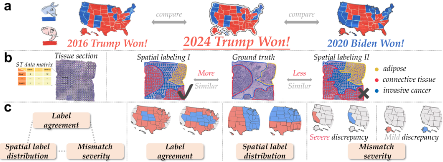
One of the most puzzling questions in the U.S. in 2024 is who, Trump or Harris, will step into the president office. The answer to this question may be explored through labeling each state's preference for Democrats (blue) or Republicans (red) on the election poll map before the Election Day and compare its similarity to those from 2016 and 2020 (Figure 1a). If it more closely resembles the 2020 map, Harris is likely favored; otherwise, Trump may prevail. This scenario exemplifies the task of spatial labeling and its similarity measurement. More formally, spatial labeling involves assigning labels to specific spatial locations (a.k.a. spatial spots) through manual assignment, spatial classification, or clustering algorithms. For instance, in pathological analysis, spatial clustering methods assign group labels to fixed spatial spots across a tissue section[Xu et al., 2024a], dissecting it into biologically distinct domains (Figure 1b) based on spot-wise gene expression profiles detected by spatial transcriptomics (ST) technologies[Dries et al., 2021]. Similarly, in epidemiological analysis of influenza at specified geographical locations [Wang et al., 2019], the primary influenza type at each location serves as its spatial label.
In scientific research, it is common to compare two spatial labelings of identical locations by measuring their similarity. For example, evaluating the effectiveness of ST classification and clustering methods requires comparing spatially labeled tissue section with the ground truth labeling[Xu et al., 2024b] (Figure 1b). Measuring similarity between spatial labels of major influenza types over time can estimate the virus' evolutionary trend and rate. Therefore, adequate measurement of spatial labeling similarity facilitates the knowledge discovery and data mining from spatial data, which should consider three aspects: label agreement, spatial label distribution, and the severity of mismatched labels. Label agreement refers to the total number of matched labels. Spatial label distribution concerns the consistency in topological structures between two spatial labelings, implying that similarity can vary with spatial organization of matches and mismatches. Mismatch severity highlights the heterogeneity in mismatches' impact on overall similarity. Using faked election poll maps as an illustration (Figure 1c), label agreement indicates the number of states favoring the same party in both maps. The impact of spatial label distribution can be seen in the dissimilarity between a horizontally split map (northern states for Democrats versus southern states for Republicans) and a vertically split map (eastern states for Democrats versus western states for Republicans). Mismatch severity means that differing in Alaska's color (3 electoral votes) is less significant than differing in California's color (55 electoral votes).
Existing methods for evaluating spatial labeling similarity can be broadly divided into two categories. The first focuses on label agreement and includes two types of methods designed for labels generated in classification and clustering tasks, referred to as supervised and unsupervised, respectively. Mathematically, assume that we have two spatial labeling results over n spots: R1 = {r : r ∈ L1 = {a1, a2, ..ak}}n and R2 = {r : r ∈ L2 = {b1, b2, ..bk′}}n , where L1 and L2 represent their respective label space. Supervised methods, applicable when the two label spaces are identical (i.e., L1 ≡ L2), include accuracy, precision, recall, and F1 score. Unsupervised methods, used when L1 ̸≡ L2 (e.g., cluster labels assigned by clustering method versus ground truth labels), include the Adjusted Rand Index (ARI) [Rand, 1971], Normalized Mutual Information (NMI) [Cover, 1999], Jaccard Score [Jolliffe and Stephenson, 2012], V-measure [Rosenberg and Hirschberg, 2007], and FowlkesMallows Index (FMI) [Halkidi et al., 2001]. They typically work by counting agreements and disagreements between pairwise spot labels. However, a significant limitation of both supervised and unsupervised methods is that they treat spatial spots independently, overlooking their spatial relationships. Consequently, they can incorrectly regard two spatial labeling results with distinct topological organizations as having high similarity. The second category comprises statistical tests like the Weisfeiler-Lehman (WL) test [Huang and Villar, 2021] and the permutation test [Welch, 1990], which are purposed for determining statistical significance of similarity without quantifying similarity level, rendering them unsuitable for this study.
Additionally, both categories treat mismatched labels equally, which, however, can differently impact the labeling similarity in practice. However, this limitation cannot be trivially addressed by assigning weights to spots because the spatial position of mismatched labels also matters. For example, in the electoral map example, Georgia and Michigan have identical weights (16 votes). However, Georgia's shift from red to blue holds more significance due to its geographical connection to other red states, signaling potential political disunity. These limitations collectively restrict the use of these methods to obtain a comprehensive, sensible, and unbiased result.
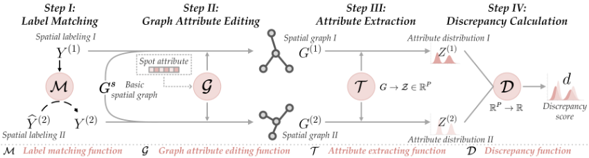
To address these limitations, we propose a methodological framework for measuring spatial labeling similarity, accounting for label agreement, spatial label distribution, and mismatching severity. The framework's workflow comprises four steps (Figure 2): Initially, if the two spatial labelings have different label spaces, they are matched to a common one using a matching function (Step I). Next, we construct a basic graph, where each spot is represented by a node positioned according to its location, with spot attributes (e.g., gene expression level) serving as node attribute. Edge types and weights are set based on the labels and attributes of the connecting nodes using a graph edit function, thereby incorporating the label matching degree and mismatching severity (Step II). In Step III, the distribution of graph attributes is estimated using an attribute extracting function. The dissimilarity of two spatial labelings is then represented by the expected discrepancy between their graph attribute distributions using a discrepancy function(Step IV). To demonstrate the efficacy of this framework, we implement it as Spatial Labeling Analogy Metric (SLAM), a novel metric for evaluating the quality of spatial labeling results and test it using both simulated and real ST data. Our main contributions include:
- Methodological Framework and Implementation. We propose a methodological framework for developing comprehensive and unbiased methods for measuring spatial labeling similarity, addressing label agreement, spatial label distribution, and mismatching severity which existing methods fail to achieve simultaneously. We further implement the framework as SLAM, an innovative spatial label-
ing evaluation metric, along with an analysis for its theoretical foundation (Appendix A.2 and A.3).
- Experimental Validation. Through deliberately designed experimental scenarios, we demonstrate that the evaluation outcomes using SLAM provide the most accurate reflection of the spatial labeling quality in ST, compared to existing metrics.
2 RelatedWork
2.1 Label Matching-BasedMethods
Labeling matching-based methods focus on the number of matched and mismatched labels between two spatial labelings, and can be divided into two categories which we refer to as supervised or unsupervised. Supervised methods require that two spatial labelings share the same label space, as explained in the Introduction section. Prevalent supervised methods include accuracy, precision, recall, and F1 score. In these methods, one spatial labeling is treated as the reference, and mismatched labels in the other labeling are considered errors to calculate the corresponding metrics. Unsupervised methods, on the other hand, do not require matched label space, instead emphasizing pairwise label agreement. That is, two locations agree if they either share the same label or not in both spatial labeling results. Common unsupervised methods include ARI, NMI, Jaccard Score, V-measure, and FMI. The ARI is an improved version of Rand index (RI), which calculates the ratio of location pairs that consistently share label or not to all possible location pairs in two spatial labelings. NMI normalizes the mutual information between two spatial labelings using their average entropies, accounting for different labeling dispersion degree and numbers, with a larger value indicating greater similarity. V-measure is equivalent to NMI, using arithmetic mean as the aggregation function. The Jaccard Score is computed as the ratio of the intersection to the union of the two sets of label pairs created from two spatial labelings. FMI takes one spatial labeling as reference and counts true positives (TPs), false positives (FPs), and false negatives (FNs) based on label agreement between the two spatial labelings. It is calculated as the geometric mean of precision and recall from TPs, FPs, and FNs. While these metrics highlight different aspects of the agreement between the two spatial labelings, they all assume that locations are equal and independent, overlooking spatial relationships and varying significance among locations, thus leading to biased evaluation results. The detailed calculation of these methods can be found in Appendix F.
2.2 Statistical Test-BasedMethods
Statistical test-based methods (e.g., WL test) typically involve computing a statistic under the null hypothesis that the two spatial labelings are independent and dissimilar. If the observed statistic value significantly deviates from the expected value, we reject the null hypothesis and believe the two spatial labeling are significantly more similar than expected by chance. The major drawback of these methods lies in their inability to quantify and compare similarity levels across labeling pairs, making them unsuitable for the objective of this study.
3 Method
3.1 Methodological Framework
Let Y (1) ∈ {a1 · · · , aK1 }n and ̂ Y (2) ∈ {b2, · · · , bK2 }n denote the label vectors of the two spatial labelings to be compared, where K1 and K2 are the total numbers of distinct labels in Y (1) and ̂ Y (2) , respectively. If Y (1) and ̂ Y (2) are in distinct label space (e.g., K1 ̸= K2), ̂ Y (2) is mapped to the space of Y (1) using a matching function M : bv → au:
Let Gs (V,Es ) represent the basic graph in Step II, where V represents the set of nodes and Es ∈ {1, 0}|ES | the set of edges. Given a spatial labeling result, its specific graph is constructed using a graph attribute editing function G, which incorporates the label distribution and, if available, spot attributes X ∈ R|V |×d , where d denotes the attribute dimension:
Here, W (∗) ∈ R|E(∗) | denotes the set of edge weights computed as per node labels (and attributes). The similarity between the two spatial labelings is estimated by comparing their graph attribute distributions, Z (1) and Z (2) , obtained using an attribute extraction function T :
The distributional discrepancy between Z (1) and Z (2) is computed using a discrepancy function D : RP → R:
Here, d is a discrepancy score, where a lower value indicates higher similarity between the two spatial labelings. Note that there are multiple choices for M, G, T , and D as per the specific context. For example, M can be the Hungarian algorithm [Mills-Tettey et al., 2007] or kernel-based probability density methods [Brbi´c et al., 2020]; ;T can be functions for calculating graph coefficients [Watts and Strogatz, 1998] or Laplacian spectrum [Chung, 1997]; while D can be functions for calculating the maximum-mean discrepancy [Gretton et al., 2012] or Wasserstein distance [Rabin et al., 2012]. In the following sections, we will give an implementation of our framework for evaluating the spatial labeling results using ST data as an example.
3.2 Application: Evaluating Spatial Labeling Result in Spatial Transcriptomics with SLAM
A common application that involves measuring spatial labeling similarity is the evaluation of spatial labeling result against ground truth labeling. To this end, we implement our framework as SLAM and test it using ST data. Spatial labeling in ST involves assigning spot labels, representing biologically distinct tissue domains, based on their locations and gene expression profiles. Specifically, an ST dataset is represented as X ∈ Rn×g , where n is the number of spots across the tissue section, g is the number of genes, and xi,j denotes gene j's expression at location i. We define the ground truth labels as Y (0) ∈ {1, 2, · · · ,K}n and a spatial labeling result as ̂ Y (1) ∈ {a1, a2..aK1 }n , contains K1 groups.
Extracting graph attribute distribution
Due to the randomness inherent to spatial labeling method, the observed annotation result Y (i) merely represents a sample from an unknown underlying distribution f (i) . Therefore, we aim to estimate f (i) given the label-conditional attributed graph G(i) (V, E(i) , W (i) ). Formally, we extract edge attributes using the function T in Equation (3), which is a one-hot encoding function here:
The edge attribute matrix of G(i) can be represented as Z (i) := [z(i) 1 , ..., z (i) |E(i) | ]T ∈ {0, 1}|E(i) |×K , where z(i) r := [z(i) r,1 , ..., z (i) r,K ]T . Z (i) is then adjusted with the edge weight matrix ̂ W (i) := [vec(W (i) )]K ∈ R|E(i) |×K to account for mismatch severity:
The density f (i) of edge attribute distribution Z (i) is then estimated using a Gaussian kernel density estimator K:
where h is the bandwidth for which a sensitivity analysis is also conducted in Appendix E.
Computing the discrepancy between graph attribute distributions
We implement the discrepancy function D in Equation (4) as a composite function of a sliced Wasserstein distance function W, a symmetric positive definite exponential kernel function Ξ, and a maximum-mean discrepancy (MMD) function ∆. The sliced Wasserstein distance function measures the discrepancy between two sample distributions of graph attributes. Since the calculation of one-dimensional Wasserstein distance has closed-form solution, sliced Wasserstein distance greatly improves the computational efficiency for multivariates [Bonneel et al., 2015], which is also empirically validated in our complexity analysis in Appendix D. The kernel function Ξ ◦ W2 is a symmetric positive definite kernel
Label matching
We implement theMfunction in Equation (1) to match ̂ Y (1) with Y (0) :
where Y (1) ∈ {1, 2, · · · ,K}n is the post-matching labels. M denotes our label matching function. Here, we propose a Jaccard coefficient-based matching algorithm as M, which can work even if K1 ̸= K (see Appendix A.1 for details).
Constructing basic spatial graph
Given a ST dataset, the basic spatial graph Gs (V, Es ) is constructed with the node set V comprising its spatial spots. In ST data such as 10x Visium, spots are typically arranged on a hexagonal grid covering the tissue slice. Thus, their spatial relationship can be naturally modeled using a mutual k-nearest neighbor graph([Dong and Zhang, 2022; Zong et al., 2022]), where the edge set Es is defined as:
where Nk(v) denotes the k-nearest neighbor set of node v. We also define a function I(u, v) : (u, v) ↦→ {1, 2, · · · , |Es |} that maps connected node pairs to edge indices.
Constructing label-conditional attributed graph
We generate labeling-specific graph G(i) , i ∈ {0, 1}, conditional on Gs , node labels Y (i) , and gene expression profiles X using a graph attribute edit function G:
Here, the types of edge E(i) are defined as:
where t ∈ {1, · · · ,K}. Additionally, W (i) ∈ R|E(i) | is introduced to account for severity variations across mislabel types. For example, a pair of similar spots of the same type should be penalized more if they are assigned distinct labels, while a pair of dissimilar spots of different types should be penalized more if they are assigned the same label. Then, we have:
where xu, xv ∼ Rg ∈ X. Sim(xu, xv) is a function measuring the similarity between attributes of nodes u and v.
and captures higher-order moments of distributional discrepancy in a uniquely-induced reproducing kernel Hilbert space (RKHS), for which we provide a detailed mathematical proof in Appendix A.2 and A.3. In this uniquely-induced RKHS, the MMD function ∆ computes the expected discrepancy between the two underlying graph attribute distributions. Put together, we have D := (∆2 ◦ Ξ ◦ W2 ) and compute the discrepancy between the underlying graph attribute distributions of the clustering result, f (1) , and the ground truth, f (0) , as d [Gretton et al., 2012]:
where x, y ∈ RK . d is then reduced to:
d =
where n0 and n1 represent the number of sampled distributions from f (0) and f (1) , respectively.
4 Experimental Design
We design seven experimental cases in which a variety of spatial labeling results of simulated and real ST datasets are evaluated using SLAM and fourteen benchmark metrics.
4.1 Experimental Cases
Label Agreement Degree. Case I: Topologically identical spatial labelings with different numbers of mislabels. An effective evaluation metric should reflect the quality change in spatial labeling due to an altered number of mislabels, even when the topological structure of the labels remains unchanged. Case II: Increased number of mislabels (Appendix C).
Consistency in Spatial Label Distribution. Case III:Mislabels at the center versus periphery. In the ground truth labeling of a tissue section in ST, spots at domain center are typically more definitive in their types than those at the domain periphery. Therefore, mislabeling domain center spots represents a more severe error with greater dissimilarity with the ground truth, which should be reflected by an effective evaluation metric. Case IV: Aggregated versus dispersed mislabels (Appendix C).
Mislabeling Severity. Case V: False positive mislabels versus false negative mislabels. In clinical diagnosis, false negatives (mislabeling a diseased spot as normal) are more serious than false positive (mislabeling a normal spot as diseased), leading to lower labeling quality. Thus, the evaluation metric should account for this asymmetry. Case VI: Mislabels with varying similarity to true labels.Mislabeling a spot to a biologically similar type (e.g., similar in gene expression profiles) is more acceptable than mislabeling it to a biologically distinct type. The evaluation metric should give a quality score consistent with this error severity gap.
Evaluating Spatial Labeling Using Real Spatial Transcriptomics Data
Case VII: Evaluating spatial labelings in a human breast cancer tissue section. To evaluate SLAM's effectiveness in practice, three unsupervised methods, including GraphST [Long et al., 2023], SpaGCN [Hu et al., 2021], and STAGATE [Dong and Zhang, 2022], are employed to label a complex breast cancer tissue section(10x-hBC-A1). SLAM evaluates these labeling results by measuring their similarity to the expert-curated ground truth labels.
4.2 Experimental Settings
Data preparation. To simplify experimental evaluation and result interpretation, we use NetworkX [Hagberg et al., 2008] to simulate the graph structures of spatial labeling results and the ground truth for all simulated cases, mimicking potential results encountered in the analysis of ST data from disease tissues.
To increase the reality of our simulated data, we use a human breast cancer 10x Visium dataset (10x-hBC-H) to match real spots to graph nodes and use real spatial gene expression to compute node similarity. For Case VI, we select 10 spots from each of the breast glands, adipose, and cancer regions in the human breast cancer 10x Visium dataset (10x-hBC-H1). In Case VII, where real spatial clustering results are obtained by applying real spatial clustering methods to the 10x-hBCA1 dataset, we follow the workflow guides provided in the original studies.
Benchmark methods. In each experimental case, we use the evaluation metrics suggested by [Yuan et al., 2024] as benchmarks. These include the supervised metrics (accuracy, precision, recall, and F1 score) and the unsupervised metrics (ARI, NMI, Jaccard Score, V-measure, and FMI) described in Section 2.1. Additionally, we include five internal metrics, which differ from SLAM and other benchmark metrics in that they do not compare the spatial labeling results with the ground truth. Instead, they evaluate the results internally based on same-label cohesion and distinct-label separation. Their inclusion ensures the comprehensiveness of our benchmarks. The calculations, ranges, and directions of all these metrics are detailed in Appendix F and Appendix G.
Evaluating SLAM and benchmark methods. We evaluate SLAM and benchmark methods from two perspectives: consistency and sensitivity. Consistency means that changes in output values should align with changes in spatial labeling quality. Sensitivity refers to the method's ability to reflect changes in spatial labeling quality. To achieve this, we design a Q coefficient, where a large positive value indicates that the corresponding metric is both consistent (positiveness) and sensitive (large value change) to changes in spatial labeling quality. Refer to Appendix B for details.
5 Results
Results of case II and IV are put in Appendix C.
5.1 Label Agreement Degree
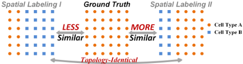
SLAM captures mislabel-induced quality change between topologically identical spatial labelings (Case I). We simulate a dataset of 36 type A spots. Spatial labeling I mislabels 24 type A spots as type B spots on the right side, while spatial labeling II mislabels 12 type A spots as type B spots on the left side (Figure 3). Despite sharing the same topological structure without considering label types, spatial labeling I and II exhibit different mislabel quantities. As a result, all internal metrics remain unchanged between the two labelings, failing to reflect the labeling quality difference due to the number of mislabels (Section 5.1). Conversely, SLAM, along with the supervised and unsupervised metrics, which are sensitive to the number of mislabels, correctly demonstrate the superiority of spatial labeling II over spatial labeling I. These results indicate SLAM's effectiveness in detecting mislabel-induced changes in result's similarity with the ground truth.
5.2 Consistency in Spatial Label distribution
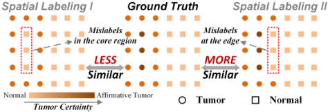
SLAM differentiates mislabels at core versus periphery regions (Case III). In pathological diagnosis, tumor core region encompasses more definitive tumor spots, whereas the tumor edge region includes plausible tumor spots that resemble adjacent normal tissues. Consequently, mislabeling tumor spots as normal in the core region is more severe and dissimilar to the ground truth compared to mislabeling those at the tumor edge. In this case, we simulate a dataset of 30 spots, with 15 circles and 15 squares representing tumor and normal spots, respectively. As shown in Figure 4, three tumor core spots are mislabeled in spatial labeling I, while three tumor edge spots are mislabeled in spatial labeling II. All supervised and unsupervised benchmark metrics demonstrate unchanged scores for the two labelings due to their insensitivity to the topological change of labels (Section 5.1). In contrast, SLAM and the five internal metrics exhibit a positive Q coefficient, indicating their ability to correctly capture the quality gap between the two spatial labelings due to changes in mislabeling locations.
5.3 Mislabeling Severity
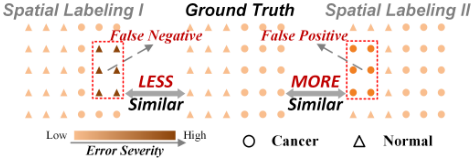
SLAM differentiates false positive and false negative errors (Case V). As explained in Section 4.1, false negatives (FNs) represent a more severe error than false positives (FPs) in clinical setting. This severity gap results in a difference in similarity with the ground truth labeling. Here, we assess whether SLAM and the benchmark metrics can capture this similarity difference. Specifically, we simulate 15 normal spots and 15 cancer spots in the ground truth labeling. Spatial labeling I includes six FNs, while spatial labeling II includes six FPs (Figure 5). The FPs and FNs are symmetrically distributed in the two labelings to eliminate topological variations. Section 5.1 shows that all benchmark metrics have zero Q values, indicating their inability to capture the difference between the two labelings, as they focus solely on the number of mislabelings or the topological structure, both of which remain unchanged across the two labelings. In contrast, SLAM's positive Q value indicates its ability to recognize that the quality of spatial labeling I is inferior to that of spatial labeling II. This is because SLAM's edge weight function (Equation (11)) assigns larger weights to edges between cancer spots, resulting in FNs being overweighted when measuring similarity with the ground truth.
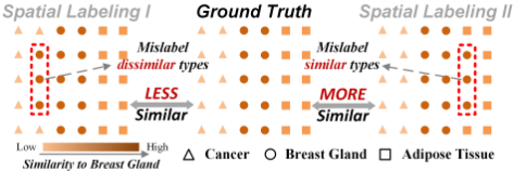
SLAM differentiates mislabels with different similarities to true labels (Case VI). In this case, the ground truth labeling comprises an equal number (10) of randomly selected spots from the adipose, breast gland, and cancer regions in the 10x-hBC-H dataset (Figure 6). Three adipose spots and three cancer spots are mislabeled as breast gland spots in spatial labeling I and II, respectively. The mislabel locations in the two spatial labelings are mirror-symmetric, ensuring that their label topological structure remains unchanged. Spots from the breast gland and adipose regions are more similar in gene expression, with an average normalized cosine similarity of 0.791, compared to 0.673 between spots from the breast gland and cancer tissues. Mislabeling breast gland spots as adipose spots leads to a labeling more similar to the ground truth than mislabeling them as cancer spots, thus a less severe error. Since spatial labeling I and II have an equal number of mislabels and identical topological structures, they differ only in mislabeling severity, which should be reflected by the evaluation metric. In Section 5.1, all metrics except SLAM exhibit unchanged scores, as indicated by their zero Q values, due to their insensitivity to mislabeling severity. SLAM, on the other hand, assigns edge weights based on the gene similarity between spots, thereby effectively capturing the labeling quality variation induced by this type of mislabeling severity.
| Case-ID | SLAM | Unsupervised | External Unsupervised | Supervised | |||||||||||
|---|---|---|---|---|---|---|---|---|---|---|---|---|---|---|---|
| ARI | NMI | Jaccard Score | FMI | V-measure | ASW | CHAOS | PAS | Internal CH Index | DB Index | Accuracy | Precision | Recall | F1 score | ||
| Label agreement degree | |||||||||||||||
| I | 0.257 | 0 | N/A | 0.166 | 0 | N/A | 0 | 0 | 0 | 0 | 0 | 0.333 | N/A | N/A | N/A |
| Consistency in spatial label distribution | |||||||||||||||
| III | 0.103 | 0 | 0 | 0 | 0 | 0 | 0.056 | 0.059 | 0.133 | 0.382 | 0.224 | 0 | 0 | 0 | 0 |
| IV * | 0.078 | 0 | N/A | 0 | 0 | N/A | 0.125 | 0.040 | 0.340 | 0.988 | 0.900 | 0 | N/A | N/A | N/A |
| Mislabeling severity | |||||||||||||||
| V | 0.110 | 0 | 0 | 0 | 0 | 0 | 0 | 0 | 0 | 0 | 0 | 0 | 0 | 0 | 0 |
| VI | 0.073 | 0 | 0 | 0 | 0 | 0 | 0 | 0 | 0 | 0 | 0 | 0 | 0 | 0 | 0 |
| Methods | SLAM↓ | ARI↑ | NMI ↑ | Jaccard Score ↑ | FMI ↑ | V-measure ↑ | ASW↑ | CHAOS ↓ | PAS ↓ | CH index ↑ | DB index ↓ |
|---|---|---|---|---|---|---|---|---|---|---|---|
| GraphST | 1.002 | 0.121 | 0.219 | 0.195 | 0.531 | 0.219 | -0.111 | 0.202 | 0.488 | 25.290 | 6.885 |
| STAGATE | 1.134 | 0.164 | 0.221 | 0.207 | 0.544 | 0.221 | -0.104 | 0.191 | 0.390 | 28.506 | 3.226 |
| SpaGCN | 1.680 | 0.032 | 0.180 | 0.143 | 0.372 | 0.180 | -0.085 | 0.240 | 0.775 | 7.224 | 12.880 |
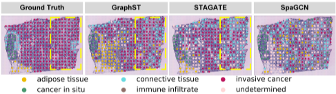
to GraphST, STAGATE generates significantly more FNs by mislabeling invasive cancer spots as connective tissue within the encircled region. Section 5.2 demonstrates that the unsupervised and internal benchmarks (except ASW) correctly reflect the inferior quality of SpaGCN compared to the other two clustering methods. However, SLAM stands out as the sole metric that identifies GraphST's superiority over STAGATE. This is likely because SLAM concurrently considers label agreement, spatial organization, and mismatch severity, offering a more comprehensive and unbiased evaluation.
5.4 Evaluating Spatial Labeling Results Using Real Spatial Transcriptomics Data (Case VII)
We evaluate SLAM's effectiveness in assessing spatial labeling results using a real human breast cancer dataset (slice A1, 10x-hBC-A1)[Andersson et al., 2020]. Since most spatial labeling methods for ST are unsupervised, we selected three well-established spatial clustering methods-SpaGCN, GraphST , and STAGATE -to generate spatial labeling results. As these methods are unsupervised, we include only unsupervised and internal metrics as benchmarks. As shown in Figure 7, the results of GraphST and STAGATE visually resemble the ground truth more closely than that of SpaGCN. A closer comparison reveals that GraphST outperforms STAGATE, particularly in terms of mismatch severity-compared
Figure 7: Case VII. Three real clustering results of 10x-hBC-A1 datasets. GraphST outperforms STAGATE within the encircled region.
6 Conclusion
We propose a methodological framework for measuring spatial labeling similarity. By accounting for all aspects of label agreement, spatial label distribution, and mismatch severity, our framework addresses the limitations of existing methods and provides a guideline for developing comprehensive and unbiased methods. Under this framework, we implement SLAM, a novel metric for evaluating spatial labeling result in ST based on its similarity to the ground truth labeling. SLAM exemplifies a concrete implementation the framework with detailed workflow steps. Through extensive carefully designed experimental cases involving both simulated and real ST data, SLAM demonstrates its superiority in accurately reflecting spatial labeling quality, highlighting the effectiveness of the proposed framework.
Acknowledgments
The project is funded by the Excellent Young Scientist Fund of Wuhan City (Grant No. 21129040740) to X.S.
Contribution Statement
Yihang Du and Jiaying Hu contributed equally.
@inproceedings{ijcai2025p562,
  title     = {A Methodological Framework for Measuring Spatial Labeling Similarity},
  author    = {Du, Yihang and Hu, Jiaying and Hou, Suyang and Ding, Yueyang and Sun, Xiaobo},
  booktitle = {Proceedings of the Thirty-Fourth International Joint Conference on
               Artificial Intelligence, {IJCAI-25}},
  publisher = {International Joint Conferences on Artificial Intelligence Organization},
  editor    = {James Kwok},
  pages     = {5047--5055},
  year      = {2025},
  month     = {8},
  note      = {Main Track},
  doi       = {10.24963/ijcai.2025/562},
  url       = {https://doi.org/10.24963/ijcai.2025/562},
}
TY - CPAPER TI - A Methodological Framework for Measuring Spatial Labeling Similarity AU - Du, Yihang AU - Hu, Jiaying AU - Hou, Suyang AU - Ding, Yueyang AU - Sun, Xiaobo T2 - Proceedings of the Thirty-Fourth International Joint Conference on Artificial Intelligence, IJCAI-25 PB - International Joint Conferences on Artificial Intelligence Organization PY - 2025 SP - 5047 EP - 5055 DO - 10.24963/ijcai.2025/562 UR - https://doi.org/10.24963/ijcai.2025/562 ER -Copied
Machine-readable versions of this paper, for tools and AI agents:





