
TCDM: A Temporal Correlation-Empowered Diffusion Model for Time Series Forecasting
Proceedings of the Thirty-Fourth International Joint Conference on Artificial Intelligence. Main Track. Pages 6732-6739.
https://doi.org/10.24963/ijcai.2025/749
Keywords
- Machine Learning: ML: Time series and data streams
- Data Mining: DM: Applications
Abstract
Although previous studies have applied diffusion models to time series forecasting, these efforts have struggled to preserve the intrinsic temporal correlations within the series, leading to suboptimal predictive outcomes. This failure primarily results from the introduction of independent, identically distributed (i.i.d.) noise. In the forward process, the addition of i.i.d. noise to the time series gradually diminishes these temporal correlations. The reverse process starts with i.i.d. noise and lacks priors related to temporal correlations, which can result in directional biases during sampling. From a frequency-domain perspective, noise disrupts the low-frequency-dominated structure of trend components, making it difficult for the model to learn long-term temporal dependencies. To address these limitations, we introduce a decomposition prediction framework to complement the novel Temporal Correlation-Empowered Diffusion Model. Overall, We decompose the time series into trend and residual components, predict them using a base model and a diffusion model, and then combine the results. Specifically, a frequency-domain MLP model was adopted as the base model due to its not distorting the original sequence, and better the capture of long-range temporal dependencies. The diffusion model incorporates two key modules to capture short- and mid-range temporal correlations: the Maintaining Temporal Correlation Module and the Redesigned Initial Module. Extensive experiments across multiple datasets demonstrate that the proposed method significantly outperforms related strong baselines.
- [Aczel and Josephy, 1991] Amir D Aczel and Norman H Josephy. The chaotic behavior of foreign exchange rates. The American Economist, 35(2):16-24, 1991.
- [Anand and Achim, 2022] Namrata Anand and Tudor Achim. Protein structure and sequence generation with equivariant denoising diffusion probabilistic models, 2022.
- [Chen et al., 2021] Minghao Chen, Houwen Peng, Jianlong Fu, and Haibin Ling. Autoformer: Searching transformers for visual recognition. In Proceedings of the IEEE/CVF in- ternational conference on computer vision, pages 12270- 12280, 2021.
- [Dhariwal and Nichol, 2021] Prafulla Dhariwal and Alex Nichol. Diffusion models beat gans on image synthesis, 2021.
- [Ho et al., 2020] Jonathan Ho, Ajay Jain, and Pieter Abbeel. Denoising diffusion probabilistic models. Advances in neural information processing systems, 33:6840-6851, 2020.
- [Jiang et al., 2023] Junji Jiang, Likang Wu, Hongke Zhao, Hengshu Zhu, and Wei Zhang. Forecasting movements of stock time series based on hidden state guided deep learn- ing approach. Information Processing & Management, 60(3):103328, 2023.
- [Kawar et al., 2021] Bahjat Kawar, Gregory Vaksman, and Michael Elad. Stochastic image denoising by sampling from the posterior distribution, 2021.
- [Li et al., 2023] Yuxin Li, Wenchao Chen, Xinyue Hu, Bo Chen, Mingyuan Zhou, et al. Transformer-modulated diffusion models for probabilistic multivariate time series forecasting. In The Twelfth International Conference on Learning Representations, 2023.
- [Li et al., 2024] Kunxi Li, Tianyu Zhan, Kairui Fu, Shengyu Zhang, Kun Kuang, Jiwei Li, Zhou Zhao, Fan Wu, and Fei Wu. Mergenet: Knowledge migration across hetero- geneous models, tasks, and modalities, 2024.
- [Liu et al., 1997] Yanhui Liu, Pierre Cizeau, Martin Meyer, C-K Peng, and H Eugene Stanley. Correlations in eco- nomic time series. Physica A: Statistical Mechanics and its Applications, 245(3-4):437-440, 1997.
- [Luo, 2022] Calvin Luo. Understanding diffusion models: A unified perspective. arXiv preprint arXiv:2208.11970, 2022.
- [Ma et al., 2024] Xiang Ma, Xuemei Li, Lexin Fang, Tian- long Zhao, and Caiming Zhang. U-mixer: An unet-mixer architecture with stationarity correction for time series forecasting. In Proceedings of the AAAI Conference on Ar- tificial Intelligence, volume 38, pages 14255-14262, 2024.
- [Meijer and Chen, 2024] Caspar Meijer and Lydia Y Chen. The rise of diffusion models in time-series forecasting. arXiv preprint arXiv:2401.03006, 2024.
- [Rasul et al., 2021] Kashif Rasul, Calvin Seward, Ingmar Schuster, and Roland Vollgraf. Autoregressive denois- ing diffusion models for multivariate probabilistic time se- ries forecasting. In International Conference on Machine Learning, pages 8857-8868. PMLR, 2021.
- [Selesnick et al., 2014] Ivan W Selesnick, Harry L Graber, Douglas S Pfeil, and Randall L Barbour. Simulta- neous low-pass filtering and total variation denoising. IEEE Transactions on Signal Processing, 62(5):1109- 1124, 2014.
- [Shen and Kwok, 2023] Lifeng Shen and James Kwok. Non- autoregressive conditional diffusion models for time se- ries prediction. In International Conference on Machine Learning, pages 31016-31029. PMLR, 2023.
- [Shen et al., 2021] Bo-Wen Shen, Roger A Pielke Sr, Xubin Zeng, Jong-Jin Baik, Sara Faghih-Naini, Jialin Cui, and Robert Atlas. Is weather chaotic?: Coexistence of chaos and order within a generalized lorenz model. Bulletin of the American Meteorological Society, 102(1):E148-E158, 2021.
- [Tashiro et al., 2021] Yusuke Tashiro, Jiaming Song, Yang Song, and Stefano Ermon. Csdi: Conditional score- based diffusion models for probabilistic time series impu- tation. Advances in Neural Information Processing Sys- tems, 34:24804-24816, 2021.
- [Walters and Heston, 1982] Roy A Walters and Cynthia He- ston. Removing tidal-period variations from time-series data using low-pass digital filters. Journal of physical oceanography, 12(1):112-115, 1982.
- [Wang et al., 2024] Qinghe Wang, Baolu Li, Xiaomin Li, Bing Cao, Liqian Ma, Huchuan Lu, and Xu Jia. Char- acterfactory: Sampling consistent characters with gans for diffusion models. arXiv preprint arXiv:2404.15677, 2024.
- [Wu et al., 2024] Likang Wu, Zhaopeng Qiu, Zhi Zheng, Hengshu Zhu, and Enhong Chen. Exploring large lan- guage model for graph data understanding in online job recommendations. In Proceedings of the AAAI Conference on Artificial Intelligence, volume 38, pages 9178-9186, 2024.
- [Xiao et al., 2021] Zhisheng Xiao, Karsten Kreis, and Arash Vahdat. Tackling the generative learning trilemma with de- noising diffusion gans. arXiv preprint arXiv:2112.07804, 2021.
- [Zeng et al., 2023] Ailing Zeng, Muxi Chen, Lei Zhang, and Qiang Xu. Are transformers effective for time series fore- casting? In Proceedings of the AAAI conference on artifi- cial intelligence, volume 37, pages 11121-11128, 2023.
- [Zheng et al., 2022] Huangjie Zheng, Pengcheng He, Weizhu Chen, and Mingyuan Zhou. Truncated diffusion probabilistic models and diffusion-based adversarial auto-encoders. arXiv preprint arXiv:2202.09671, 2022.
References were extracted automatically from the PDF and may contain errors.
Full text extracted automatically from the PDF; figures, tables and equations may differ. The PDF is the version of record.
1 Introduction
Time series forecasting is a fundamental task that is crucial in many areas, such as financial markets [Aczel and Josephy, 1991; Jiang et al., 2023] and weather systems [Shen et al., 2021]. Specifically, time series are sequences composed of points that are temporally correlated and numerically related. As an essential characteristic of time series, temporal correlation, also known as temporal dependence, refers to the relationship between different points over time [Liu et al., 1997; Wu et al., 2024] and is crucial for making accurate predictions [Zeng et al., 2023; Li et al., 2024]. Moreover, Time series forecasting can be viewed as a generative task that generates a prediction sequence conditioned on a historical sequence. As state-of-the-art generative models, diffusion models-known for their remarkable success in fields like computer vision [Dhariwal and Nichol, 2021; Kawar et al., 2021] and computational chemistry [Anand and Achim, 2022]-have been naturally introduced to the task of time series forecasting.
Recent research on diffusion models for time series forecasting [Rasul et al., 2021; Tashiro et al., 2021; Shen and Kwok, 2023; Li et al., 2023] has shown promising results. Nevertheless, as will be empirically demonstrated in our experimental section 4.3, diffusion methods often fail to effectively preserve the intrinsic temporal dependencies of time series [Ma et al., 2024], naturally leading to a decline in modeling performance. This shortcoming can be attributed to the independent and identically distributed (i.i.d.) Gaussian noise. Due to stochasticity, in the forward process, adding Gaussian noises over too many diffusion steps makes each time point approach independent Gaussian distribution, which can intuitively result in the disappearance of temporal correlation. In the reverse processes, these models typically start from i.i.d. noise, which lacks prior knowledge of temporal dependencies during sampling, resulting in generated time series with insufficient temporal correlation.
Meanwhile, due to the aforementioned properties of the diffusion model, not all components of time series data are well-suited for prediction using diffusion model [Selesnick et al., 2014]. In particular, the trend component, extracted using the classical Moving Average method [Chen et al., 2021], exhibits smooth variations, with energy primarily concentrated in the low-frequency domain, thereby reflecting long-term temporal dependencies [Zeng et al., 2023; Chen et al., 2021]. However, the addition of noise can disrupt its temporal correlation. From a frequency domain perspective, adding noise with a uniform frequency distribution is equivalent to introducing significant high-frequency energy into a predominantly low-frequency signal [Walters and Heston, 1982]. This interference hinders the model's ability to learn low-frequency features, thereby affecting the output's long-term temporal dependencies.
To address these challenges, we introduce a decomposition prediction framework to complement the Temporal Correlation-Empowered Diffusion Model, together referred to as TCDM. The framework adopts the divide-and-conquer approach. It begins by decomposing the time series into two components: a trend component and a residual component. For the trend component, characterized by long-term temporal correlations and energy concentrated in the low-frequency domain, we utilize a frequency-domain MLP-based model. This model more easily learns compact low-frequency representations, thereby enhancing its ability to effectively capture long-term temporal dependencies. The residual component, containing significant noise and seasonal information, primarily reflecting short- and mid-range temporal dependencies, is processed using a diffusion model. The diffusion model is utilized for its strong generative and denoising capabilities, while the residual component's broad spectral distribution ensures stable resistance to noise during diffusion training.
Specifically, during the forward process of diffusion, we introduce the Maintaining Temporal Correlation Module. This module is designed to handle the noise added at each time step ensuring that the model can still learn temporal correlations even at larger diffusion step. Concurrently, during the reverse process sampling, we specifically design the variance to continuously steer towards preserving temporal correlations. Meanwhile, fewer diffusion steps in the reverse process help maintain the internal temporal correlations of the data more effectively. By redesigning the initial state of the reverse process, achieved by truncating the diffusion process, we enhance the preservation of internal temporal correlations. This strategy also reduces the number of steps required in both the forward and reverse process.
In this work,we introduce a decomposition-based predictive framework to complement the novel temporal correlation-empowered diffusion model for multivariate time series forecasting. Our experiments across various real-world datasets demonstrate that the model achieves state-of-the-art performance. Our contributions are summarized as follows:
- We propose an innovative decomposition framework for multivariate time series forecasting that integrates a base model with a diffusion model to capture long-term and short-term temporal dependencies separately.
- We focus on the overall design of the temporal correlation in the diffusion model, which is divided into three key aspects: noise addition, initial state, and the sampling process. Each element is strategically implemented to improve the preservation of temporal correlations throughout the model.
- We demonstrate the state-of-the-art performance of proposed method through experiments on various realworld multivariate time series forecasting datasets.
2 Background
2.1 Denoising diffusion probabilistic models
Diffusion models comprise a forward diffusion process and a backward denoising process. Beginning with the widely recognized denoising diffusion probabilistic model [Ho et al., 2020]. The data distribution x0 ∼ q(x0) is defined along with a Markovian noising process q that gradually adds noise to the data x0 to produce noised samples xT . Specifically, each step of the noising process adds Gaussian noise according to a variance schedule given by βt:
Furthermore, q(xt | x0) can be expressed as a Gaussian distribution. With αt := 1 -βt and ¯αt := ∏ts=0 αs,
It is sufficient to train a neural network to predict a mean µθ:
To train this model such that p(x0) learns the true data distribution q(x0), the model can be trained by optimizing the variational lower bound Lvlb for pθ(x0). Training µθ(xt, t) and training ϵθ(xt, t) are equivalent [Luo, 2022]. They demonstrated that predicting the noise added at each step is effectively the same as predicting x0 at each step. Rather than directly parameterizing µθ(xt, t) as a neural network, the methodology involves training the model ϵθ(xt, t) to predict the noise ϵ. The corresponding simplified objective is given by:
The mean µθ(xt, t) can also be derived using a denoising network xθ, which estimates the clean data x0 given xt. This estimate xθ(xt, t) allows the following expression for µθ(xt, t) to be set:
The parameter θ is then optimized by minimizing the loss function as below:
3 Method
The key components of our model include: (i) Decomposition of Time Series, (ii) Maintaining Temporal Correlation Module, and (iii) Redesigned Initial Module.
3.1 ProblemFormulation
When using a diffusion model for time series forecasting, our objective is to predict future values y0 1:F ∈ RC×F based on the observed historical data x1:H ∈ RC×H , where x1:H (denoted as X) is defined as {x1, x2, . . . , xH | xt ∈ RC }. and y0 1:F (denoted as Y0 ) is defined as {y0 1 , y0 2 , . . . , y0F | y0 t ∈ RC }. The superscript t in yt1:F denotes that these values are at the t-th step of diffusion. Thus, y0 1:F , the superscript 0 indicates that they are at the 0-th step of the diffusion process, meaning these are the true values before any noise is added. The conditioning of diffusion models for time-series [Shen and Kwok, 2023] can be done by conditioning the generation of the forecast through the reverse process on historical data, as follows:
where c is the condition, c = F (x1:H) and F is a conditional network.
3.2 Overview of TCDM
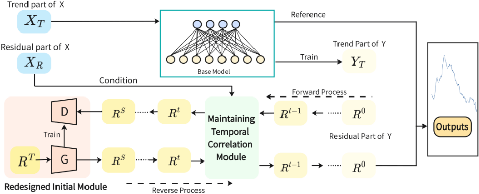
As depicted in Figure 1, during the training process, the target Y0 is initially decomposed into the trend component Y0T and the residual component Y0R, also denoted as R0 . Similarly, X is decomposed into XT and XR. The Base Model employs XT to predict the trend component Y0T . Concurrently, the residual component R0 is predicted using a diffusion model conditioned on XR. The diffusion model integrates the Maintaining Temporal Correlation Module and the Redesigned Initial Module. The predictive outputs from diffusion model are combined with those from the Base Model to generate the final results.
3.3 Decomposition of Time Series
Given that time series are generally modeled as a combination of trend, seasonal, and noise components, we refer to the seasonal and noise components as the residuals. The addition of noise can disrupt the intricate relationships within the data. To address this, we extract the more predictable trend component using the classical seasonal-trend decomposition technique described by wu2021autoformer.
the data point at the ith time step is denoted by y0 i . The trend component, represented as ˜ y0 i , is computed as a moving average within a fixed-length time window, effectively capturing the underlying trend of the time series. The residual component, denoted by ∆y0 i , captures the cyclical variations and the influence of noise after the trend has been removed. Similarly, the lookback window X is also decomposed. The model uses the trend part of X to predict the trend part of the target Y0 , and the residual part of X to predict the residual part of Y0 . This approach help to ensure consistency between the training and prediction data.
Base Model Selection
The moving average can be viewed as the convolution of the input signal Y 0 with a uniform filter h[n]. The uniform filter is defined as:
Therefore, the output of the moving average can be expressed as:
Proposition 1. A symmetric moving average filter in the time domain is equivalent to a low-pass filter in the frequency domain.
The proof is provided in the Appendix.
In the frequency domain, trend components are characterized by energy concentrated in the low-frequency region of the spectrum. When training a frequency-domainbased MLP, the input features primarily capture this valuable low-frequency information, allowing the model to effectively learn these features. Therefore, theoretically, a frequency-domain-based MLP model is more suitable for trend component forecasting. Experimentally, as shown in the Appendix, we compare the predictive performance of a frequency-domain-based MLP, a time-domain-based MLP, and a transformer-based model. The results demonstrate that the frequency-domain-based MLP outperforms the others. The detailed structure of the Base Model is also provided in the Appendix.
After obtaining the prediction model for the trend component, we proceeded to design a diffusion model for predicting the residual component. Due to the complexity of these cyclical patterns and the uncertainty of noise, the residual component is a key factor that affects the accuracy of time series predictions.
3.4 Maintaining Temporal CorrelationModule
We use the Residual part of Y: R0 as the initial state of the forward process in the diffusion model,thus it also serves as the output of the diffusion model. Then for the transition equation utilized during sampling, pθ(Rt-1 | Rt ,R0) = N(Rt-1 ; µθ(Rt , t),Σθ(Rt , t)), where µθ(Rt , t) is formulated as √αt(1-¯αt-1) 1-¯αt Rt + √ ¯αt-1βt 1-¯αt Rθ(Rt, t), with Rθ(Rt, t) representing the trained diffusion network. Our Temporally Correlated Noise is specifically designed for µθ(Rt , t), and accordingly, the Sampling Towards Temporal Correlation is tailored for Σθ(Rt , t).And details on the initial state of sampling presented in the Redesigned Initial Module.
Temporal Correlated Noise in Forward Process
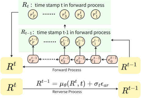
For the target data Rt = rt1:F , composed of time points rt1 , rt2 , . . . , rtF , during the forward diffusion process, the noise added at diffusion step t to the i th data point rt-1 i is denoted by ϵti :
We propose the introduction of temporally correlated noise during the forward process, enabling the model to learn more temporal correlations even for larger diffusion step t. That means µθ(Rt , t) will exhibit temporal correlation during the sampling process.
Our noise design emulates the method of noise addition used in diffusion models as referenced in Equation 1. We have modeled the noise as a Markov process (first-order autoregressive process) where the noise for the next time point i is based on the noise at the current time point i -1, with new random variations introduced at each subsequent time point. The noise added at time t to the ith timestep data point rt-1 i is denoted by ϵti .
The variance design mentioned above ensures that Var(ϵti ) remains constant at 1, ensuring that the noise level added at each time point within the target window is the same as i increases.
This design ensures that as the diffusion step t increases, a correlation is maintained within the same target window , even when t becomes large. Although this correlation is intentionally engineered, when λi is set appropriately, the Temporal Correlated Noise forces the model to preserve local correlations between consecutive data points, enabling the model to automatically adjust to the correct correlations.
Sampling Towards Temporal Correlation
Following the precedent set by [Ho et al., 2020], Σθ(Rt , t) is typically configured as σ2 t I, then
This formulation models the transition fromRt to Rt-1 , with the noise variance governed by σ2 t . Our objective in the reverse process is to impart temporal correlation priors to the model. Our optimization goal is to minimize the KL divergence DKL(q(Rt-1|Rt,R0)∥pθ(Rt-1|Rt)). To echo the noise in the forward process, during the sampling phase, we adjust the zt values to facilitate sampling in a direction that respects the sequence correlations. Consequently, we define:
where ϵti is sampled by Equation 12, transforming the sampling equation as follows:
this approach ensures that the sampling process is optimally aligned with the inherent temporal dynamics of the sequence.
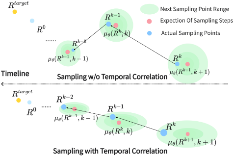
As illustrated in Figure 3, the top panel presents the scenario 'without Maintaining Temporal Correlation Module', where the sampled µθ(Rt , t) can exhibit significant fluctuations due to the absence of guidance on temporal correlations. In this scenario, zt adheres to a standard normal distribution, leading to a spherical sampling range that signifies indiscriminate sampling across all directions. Conversely, the bottom panel, labeled 'with Maintaining Temporal Correlation Module', depicts µθ(Rt , t) being influenced by noise specifically tailored for temporal correlations, which directs the sampling towards Rtarget . The design of ϵar in this scenario makes the sampling range elliptical, enhancing sampling along the axes of temporal correlations. Thus, the final sampled outcome R0 is more likely to closely approximate Rtarget , resulting in superior generative results.
3.5 Redesigned Initial Module
Instead of relying on manually designed functions, we suggest halting the diffusion process before it reaches a state close to pure noise and then initiating the reverse process from that point. By doing so, the initial state of the reverse process retains the natural temporal correlations inherent in the time series, rather than those imposed by artificial design.
When truncating the diffusion process at time S, the forward process is halted at RS . Therefore, we maintain the original noise schedule {β1, β2, . . . , βT} and select the subset {β1, β2, . . . , βS+1} as the new noise schedule[Zheng et al., 2022]. This approach retains the remaining original diffusion process. Since RS has not fully diffused into a noisedominated state, reverse sampling from Gaussian noise is infeasible. To address this issue, a generator is necessary to obtain the data distribution at S. This is accomplished using a Generative Adversarial Network (GAN) [Xiao et al., 2021].
During the reverse process, a generator Gϕ is required to produce RS , such that RS = Gϕ(z), where z ∼ N(0, I). If we approximate q(RS+1 | RS ) ≈ q(RT ) and q(RT ) ∼ N(0, I), then
This can be interpreted as enabling the diffusion model to use RT to reach RS with one step of the reverse process[Wang et al., 2024]. Therefore, the optimization objective is to minimize the KL divergence between the prior distribution of the forward process q(RS ) and the posterior distribution pϕ(RS ) , where RS is generated in one step by the generator
Referring to Equation 6, since the preserved parts of the diffusion process remain unchanged, our new loss function is defined as:
This represents the final version of the loss function for the diffusion model, where Lt (θ) is set as the version predicting the initial value R0 . The generator Gϕ is adversarially optimized using a discriminator Dψ, details of Dψ are provided in the appendix. The optimization objective LS (ϕ)is as follows:
Therefore, the denoising network of the diffusion model is trained using Rt , with the diffusion step t as input and XR as a condition, aiming to output Rt-1 . This denoising network also acts as the generator G for the reverse process, hence during training, we employ adversarial training of the denoising network and the discriminator D. Once trained, during inference, Gaussian noise RT is inputted into G, which generates predictions RS . These are then iteratively sampled through the Maintaining Temporal Correlation Module to eventually produce the predicted YR, which, when combined with the Base Model's predicted YT , yields the final outputs.
4 Experiments
4.1 Experiment Setup
We conducted experiments on 9 public datasets [Meijer and Chen, 2024], including NorPool, Caiso, Traffic, Electricity, Weather, Exchange, ETTh1, ETTm1, and Wind. Each of these datasets comprises multivariate time series. Detailed descriptions and Implementation Details are provided in Appendix. The history length, chosen from the set of (96, 192, 336, 720), and 1440 based on the validation set performance, informs the model's temporal context. A prediction length of 168 was selected for the ETTm1, Wind, Traffic, Electricity, ETTh1, and Exchange datasets. For the NorPool and Caiso datasets, a longer prediction length of 720 was opted to accommodate their unique temporal dynamics.
Evaluation Metrics
Following previous studies, the experiments utilized Mean Squared Error (MSE) to measure the predictive performance of the models. To ensure the results' convincing nature, we averaged the results over 10 runs for each experiment.
4.2 Overall Performance
Table 1 shows the results of multivariate predictions. Nonautoregressive diffusion models TimeDiff for time series have strong predictive abilities, suggesting that diffusion models are promising. Our method outperforms not only existing diffusion-based ones but also other baselines. It shows significant improvement on complex datasets like ETTm1 and ETTh1. Time series decomposition helps the model understand the data better. However, for Casio and Traffic, the obvious periodicity of the sequences may cause additional errors when time series decomposition is used. Our model achieved the best results across six datasets, demonstrating its advanced capabilities. Details of the model and additional result visualizations are provided in the Appendix.
| NorPool | Caiso | Weather | ETTm1 | Wind | Traffic | Electricity | ETTh1 | Exchange | Avg Rank | |
|---|---|---|---|---|---|---|---|---|---|---|
| Our Model | 0.655 (1) | 0.132 (2) | 0.211 (1) | 0.323 (1) | 0.881 (2) | 0.445 (2) | 0.161 (1) | 0.396 (1) | 0.160 (1) | 1.333 (1) |
| TimeDiff | 0.664 (2) | 0.138 (4) | 0.219 (4) | 0.330 (3) | 0.875 (1) | 0.449 (3) | 0.172 (5) | 0.405 (2) | 0.169 (4) | 3.111 (2) |
| TimeGrad | 1.105 (14) | 0.242 (12) | 0.308 (13) | 0.479 (11) | 1.052 (11) | 0.674 (9) | 0.253 (12) | 0.612 (12) | 0.290 (9) | 11.444 (12) |
| CSDI | 0.801 (10) | 0.191 (7) | 0.280 (9) | 0.477 (10) | 1.045 (10) | - | - | 0.497 (8) | 0.261 (7) | 8.714 (8) |
| SSSD | 0.748 (7) | 0.208 (9) | 0.275 (8) | 0.430 (9) | 1.016 (9) | 0.721 (10) | 0.225 (10) | 0.561 (11) | 0.301 (11) | 9.333 (9) |
| D3VAE | 0.765 (9) | 0.238 (11) | 0.291 (10) | 0.351 (7) | 1.013 (8) | 0.781 (13) | 0.206 (8) | 0.504 (10) | 0.316 (13) | 9.889 (10) |
| FreTS | 0.669 (3) | 0.135 (3) | 0.225 (6) | 0.328 (2) | 0.895 (4) | 0.470 (5) | 0.170 (4) | 0.425 (4) | 0.162 (2) | 3.667 (3) |
| TimesNet | 0.682 (6) | 0.130 (1) | 0.215 (2) | 0.341 (5) | 0.905 (6) | 0.601 (6) | 0.172 (6) | 0.433 (7) | 0.221 (6) | 5.000 (6) |
| PatchTST | 0.671 (4) | 0.139 (6) | 0.224 (5) | 0.333 (4) | 0.891 (3) | 0.464 (4) | 0.165 (2) | 0.430 (6) | 0.165 (3) | 4.111 (4) |
| iTransformer | 0.675 (5) | 0.138 (5) | 0.217 (3) | 0.344 (6) | 0.899 (5) | 0.437 (1) | 0.168 (3) | 0.428 (5) | 0.170 (5) | 4.222 (5) |
| FedFormer | 0.752 (8) | 0.205 (8) | 0.272 (7) | 0.389 (8) | 1.012 (7) | 0.609 (7) | 0.205 (7) | 0.417 (3) | 0.267 (8) | 7.000 (7) |
| Autoformer | 0.836 (11) | 0.226 (10) | 0.302 (11) | 0.513 (13) | 1.083 (13) | 0.615 (8) | 0.212 (9) | 0.498 (9) | 0.302 (12) | 10.667 (11) |
| Pyraformer | 0.972 (12) | 0.273 (14) | 0.305 (12) | 0.494 (12) | 1.061 (12) | 0.745 (11) | 0.257 (13) | 0.641 (14) | 0.322 (14) | 12.667 (13) |
| Informer | 0.980 (13) | 0.242 (13) | 0.315 (14) | 0.541 (14) | 1.168 (14) | 0.779 (12) | 0.250 (11) | 0.625 (13) | 0.298 (10) | 13.000 (14) |
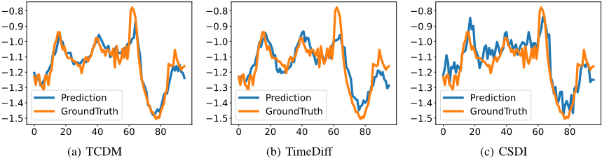
Additionally, we selected a portion of the prediction results for demonstration. As shown in Figure 4, our method aligns more closely with the actual temporal values on the ETTm1 dataset compared to other methods. This chart illustrates the differences between non-autoregressive diffusion models, represented by TimeDiff, and autoregressive diffusion models, exemplified by CSDI. CSDI suffers from error accumulation, leading to subpar predictions, especially in capturing significant peaks. TimeDiff addresses the issue of error accumulation but fails to adequately model the internal correlations within the sequence. Our TCDM can predict values across different timestamps very accurately. This further demonstrates the effectiveness of our method in capturing seasonal and trend patterns.
4.3 Designing Criteria to Validate the Temporal Correlation of Predicted Series
For the predicted series YP and the actual series YT , we aim to quantitatively measure the difference in their temporal correlations. Initially, we compute the partial autocorrelation coefficients for each feature channel i within the range {1, . . . ,D}. Employing partial autocorrelation coefficients is advantageous as they mitigate the confounding influences of intermediate variables, thus more precisely delineating the direct relationships between two variables. Using the mean squared error helps to limit the disproportionate impact of any single channel. Given a specific lag value k, the partial autocorrelation coefficients for both series are calculated and denoted by ϕi,k P and ϕi,k T , respectively. After setting amaximum lag value E, we can generate the arrays [ϕi,1 P , ϕi,2 P , . . . , ϕi,E P ] and [ϕi,1 T , ϕi,2 T , . . . , ϕi,E T ]. The index, calculated as
We propose and refer to it as the Normalized Partial Autocorrelation Difference Index (N-PADI). A lower N-PADI value indicates that the predicted series effectively captures the temporal correlations of the actual series. From the data presented in Table 2, it is evident that the performance of N-PADI is heavily influenced by its use of the L2 distance, which significantly affects the accuracy of temporal capture. TimeGrad faces challenges in grasping temporal correlations within time series. Another diffusion-based model, TimeDiff, achieves better MSE performance compared to FreTS. However, the noise-adding mechanism inherent to diffusion models, combined with the extended forward step t, limits its ability to capture temporal correlations, leading to higher N-PADI values than FreTS. PatchTST, a transformerbased model, also fails to learn additional temporal correlations compared to FreTS, underscoring the limitation of transformers in effectively retaining temporal correlations even with positional embeddings. Conversely, TCDM, our nonautoregressive diffusion model, incorporates the Maintaining Temporal Correlation Module and the Redesigned Initial Module, which significantly aid in preserving temporal correlations, thereby improving predictive performance.
| TCDM | TimeDiff | FreTS | TimeGrad | PatchTST | |
|---|---|---|---|---|---|
| ETTh1 | 0.559 | 60.057 | 0.581 | 80.012 | 4.527 |
| ETTm1 | 4.972 | 56.954 | 5.041 | 60.097 | 14.664 |
4.4 Hyperparameter Analysis
Truncated Timestamp
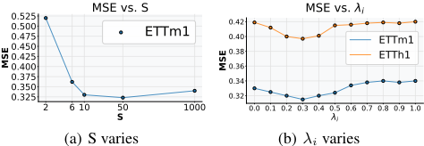
The experiment was conducted on the ETTh1 dataset. As shown in Figure 5, when S = 2, the generator struggles to learn effectively due to the limited number of diffusion steps, resulting in poor performance. However, as S increases from 2 to 50, the additional diffusion steps enable the generator to acquire more precise knowledge, significantly improving the quality of the generated initial states. This suggests that at S = 50, the model is capable of producing fairly realistic RS . Comparing S = 50 to S = 1000, S = 50 places the model in a better initial state. Furthermore, when the diffusion step exceeds 100, it becomes difficult to learn effective knowledge, including temporal correlations, highlighting the effectiveness of the Redesigned Initial Module.
Settings of Maintaining Temporal Correlation Module λi
From Figure 5, it is observed that on both datasets, as λi increases, the MSE initially decreases and then increases, with the minimum point reached at 0.3. This pattern may be attributed to both ETTh1 and ETTm1 being excerpts from the ETT dataset. As λi ranges from 0 to 0.3, the Temporal Coherent Noise Module gradually aids the model in better capturing the relationships within the time series. Although the relationships are artificially defined, they can guide the model to autonomously learn the true event correlations. However, when λi increases beyond 0.3, overfitting occurs. This is due to the Temporal Coherent Noise Module excessively modeling the artificially designed temporal correlations, which impedes the model's ability to learn authentic correlations, resulting in a decline in predictive performance.
4.5 Ablation Study
We maintain consistency with the hyperparameters of the main experiment and conduct ablation studies to validate individual model effectiveness. We perform these module ablation experiments in a multivariate setting on the ETTh1 and Exchange datasets.
As shown in Table 3, ablation studies on the TCDM model demonstrate that the full TCDMmodule consistently outperforms configurations with any single module removed across datasets, indicating a synergistic enhancement of overall performance. Removing the Maintaining Temporal Correlation Module led to significant declines in performance on the Exchange, underscoring its crucial role in predictive accuracy. The Redesigned Initial Module proved especially effective on ETTh1, enhancing prediction precision for dynamic patterns. Although removing the Time Series Decomposition had a minor overall impact, it increased the error on the Exchange dataset (from 0.160 to 0.185), highlighting its importance for temporally coherent data. These findings emphasize the critical contributions of each module to achieving high accuracy in multivariate time series forecasting.
| Module | ETTh1 | Exchange |
|---|---|---|
| Full TCDM | 0.396 | 0.160 |
| w/o MTC Module | 0.403 | 0.190 |
| w/o Redesigned Initial Module | 0.406 | 0.171 |
| w/o Decomposition of Time Series | 0.402 | 0.185 |
5 Conclusion
In this study, we propose a novel decomposition-based prediction framework to enhance the Temporal CorrelationEmpowered Diffusion Model, collectively referred to as TCDM. The framework leverages time series decomposition to integrate a base model with a diffusion model, enabling it to effectively capture both long-term and short-term temporal dependencies. The diffusion model is specifically designed to preserve temporal correlations through two key components: the Maintaining Temporal Correlation Module and the Redesigned Initial Module. These components are developed by addressing three critical aspects of diffusion models: noise addition, initial state, and the sampling process. Experimental results demonstrate that each component contributes to improved model performance, and TCDM significantly surpasses existing models, establishing it as a powerful and reliable solution for accurate time series prediction.
@inproceedings{ijcai2025p749,
  title     = {TCDM: A Temporal Correlation-Empowered Diffusion Model for Time Series Forecasting},
  author    = {Xu, Huibo and Wu, Likang and Wang, Xianquan and Liu, Zhiding and Liu, Qi},
  booktitle = {Proceedings of the Thirty-Fourth International Joint Conference on
               Artificial Intelligence, {IJCAI-25}},
  publisher = {International Joint Conferences on Artificial Intelligence Organization},
  editor    = {James Kwok},
  pages     = {6732--6739},
  year      = {2025},
  month     = {8},
  note      = {Main Track},
  doi       = {10.24963/ijcai.2025/749},
  url       = {https://doi.org/10.24963/ijcai.2025/749},
}
TY - CPAPER TI - TCDM: A Temporal Correlation-Empowered Diffusion Model for Time Series Forecasting AU - Xu, Huibo AU - Wu, Likang AU - Wang, Xianquan AU - Liu, Zhiding AU - Liu, Qi T2 - Proceedings of the Thirty-Fourth International Joint Conference on Artificial Intelligence, IJCAI-25 PB - International Joint Conferences on Artificial Intelligence Organization PY - 2025 SP - 6732 EP - 6739 DO - 10.24963/ijcai.2025/749 UR - https://doi.org/10.24963/ijcai.2025/749 ER -Copied
Machine-readable versions of this paper, for tools and AI agents:





