
Dynamic Anchor-based Ensemble Clustering via Hypergraph Reconstruction
Proceedings of the Thirty-Fourth International Joint Conference on Artificial Intelligence. Main Track. Pages 6740-6748.
https://doi.org/10.24963/ijcai.2025/750
Keywords
- Machine Learning: ML: Clustering
- Machine Learning: ML: Ensemble methods
Abstract
Ensemble clustering learns a consensus result by integrating a set of base clustering results. Recently, anchor-based methods construct an anchor similarity matrix to represent the affinity relationships among samples, significantly improving computational efficiency. However, these methods struggle with fixed anchors generated by static anchor learning strategies, which lead to low-quality anchor similarity matrix and poor clustering accuracy. To address this issue, we propose a novel method named dynamic anchor-based ensemble clustering via hypergraph reconstruction (YACHT). Specifically, YACHT first transforms the base clustering results into a hypergraph and designs a novel hypergraph enhancement strategy to improve the reliability of the initial hypergraph. YACHT reconstructs the hypergraph through matrix factorization and introduces a mapping matrix to filter out redundant information, capturing a high-quality anchor similarity matrix. Then, YACHT attempts to incorporate the hypergraph into the optimization objective to achieve hypergraph updates. To ensure the accuracy of hypergraph updates, we impose a hypergraph regularizer and a local consensus information alignment term. The alignment term is implemented by minimizing the discrepancy between the label partition derived from the hypergraph regularizer and the local consensus information indicator matrix extracted from the base clustering results. Extensive experimental results demonstrate the outstanding performance of the proposed YACHT. The code is available at https://github.com/scu-kdde/YACHT.
- [Abbasi et al., 2019] Sadr-olah Abbasi, Samad Nejatian, Hamid Parvin, Vahideh Rezaie, and Karamolah Bagher- ifard. Clustering ensemble selection considering quality and diversity. Artificial Intelligence Review, 52(2):1311- 1340, 2019.
- [Bai et al., 2020] Liang Bai, Jiye Liang, and Fuyuan Cao. A multiple k-means clustering ensemble algorithm to find nonlinearly separable clusters. Information Fusion, 61:36- 47, 2020.
- [Bazaraa et al., 2013] Mokhtar S Bazaraa, Hanif D Sherali, and CM Shetty. Nonlinear Programming: Theory and Al- gorithms. John Wiley & Sons, 2013.
- [Chen et al., 2023] Man-Sheng Chen, Jia-Qi Lin, Chang- Dong Wang, Wu-Dong Xi, and Dong Huang. On reg- ularizing multiple clusterings for ensemble clustering by graph tensor learning. In Proceedings of the 31st ACM In- ternational Conference on Multimedia, pages 3069-3077, 2023.
- [Feng et al., 2024] Wenyi Feng, Zhe Wang, Ting Xiao, and Mengping Yang. Adaptive weighted dictionary represen- tation using anchor graph for subspace clustering. Pattern Recognition, 151:110350, 2024.
- [Fern and Brodley, 2004] Xiaoli Zhang Fern and Carla E Brodley. Solving cluster ensemble problems by bipartite graph partitioning. In Proceedings of the 21st Interna- tional Conference on Machine Learning, page 36, 2004.
- [Gao et al., 2022] Yue Gao, Zizhao Zhang, Haojie Lin, Xibin Zhao, Shaoyi Du, and Changqing Zou. Hypergraph learning: Methods and practices. IEEE Transactions on Pattern Analysis and Machine Intelligence, 44(5):2548- 2566, 2022.
- [Hao et al., 2024] Zhezheng Hao, Zhoumin Lu, Guoxu Li, Feiping Nie, Rong Wang, and Xuelong Li. Ensemble clustering with attentional representation. IEEE Trans- actions on Knowledge and Data Engineering, 36(2):581- 593, 2024.
- [Huang et al., 2016] Dong Huang, Jian-Huang Lai, and Chang-Dong Wang. Robust ensemble clustering using probability trajectories. IEEE Transactions on Knowledge and Data Engineering, 28(5):1312-1326, 2016.
- [Huang et al., 2018] Dong Huang, Chang-Dong Wang, and Jian-Huang Lai. Locally weighted ensemble cluster- ing. IEEE Transactions on Cybernetics, 48(5):1460-1473, 2018.
- [Huang et al., 2020] Dong Huang, Chang-Dong Wang, Jian- Sheng Wu, Jian-Huang Lai, and Chee-Keong Kwoh. Ultra-scalable spectral clustering and ensemble clustering. IEEE Transactions on Knowledge and Data Engineering, 32(6):1212-1226, 2020.
- [Huang et al., 2021] Dong Huang, Chang-Dong Wang, Hongxing Peng, Jianhuang Lai, and Chee-Keong Kwoh. Enhanced ensemble clustering via fast propagation of cluster-wise similarities. IEEE Transactions on Systems, Man, and Cybernetics: Systems, 51(1):508-520, 2021.
- [Huang et al., 2023] Qirui Huang, Rui Gao, and Hoda Akha- van. An ensemble hierarchical clustering algorithm based on merits at cluster and partition levels. Pattern Recogni- tion, 136:109255, 2023.
- [Jia et al., 2021] Yuheng Jia, Hui Liu, Junhui Hou, and Qingfu Zhang. Clustering ensemble meets low-rank tensor approximation. In Proceedings of the AAAI Conference on Artificial Intelligence, volume 35, pages 7970-7978, 2021.
- [Jia et al., 2024] Yuheng Jia, Sirui Tao, Ran Wang, and Yongheng Wang. Ensemble clustering via co-association matrix self-enhancement. IEEE Transactions on Neu- ral Networks and Learning Systems, 35(8):11168-11179, 2024.
- [Li et al., 2021] Feijiang Li, Yuhua Qian, and Jieting Wang. Got: A growing tree model for clustering ensemble. In Proceedings of the AAAI Conference on Artificial Intelli- gence, volume 35, pages 8349-8356, 2021.
- [Li et al., 2023] Hongmin Li, Xiucai Ye, Akira Imakura, and Tetsuya Sakurai. Lsec: Large-scale spectral ensemble clustering. Intelligent Data Analysis, 27(1):59-77, 2023.
- [Li et al., 2024] Taiyong Li, Xiaoyang Shu, Jiang Wu, Qingxiao Zheng, Xi Lv, and Jiaxuan Xu. Adaptive weighted ensemble clustering via kernel learning and lo- cal information preservation. Knowledge-Based Systems, 294:111793, 2024.
- [Liang et al., 2020] Yinian Liang, Zhigang Ren, Zongze Wu, Deyu Zeng, and Jianzhong Li. Scalable spectral ensemble clustering via building representative co-association ma- trix. Neurocomputing, 390:158-167, 2020.
- [Liu et al., 2015] Hongfu Liu, Tongliang Liu, Junjie Wu, Dacheng Tao, and Yun Fu. Spectral ensemble clustering. In Proceedings of the 21th ACM SIGKDD International Conference on Knowledge Discovery and Data Mining, pages 715-724, 2015.
- [Liu et al., 2024] Suyuan Liu, Ke Liang, Zhibin Dong, Siwei Wang, Xihong Yang, Sihang Zhou, En Zhu, and Xinwang Liu. Learn from view correlation: An anchor enhance- ment strategy for multi-view clustering. In Proceedings of the IEEE/CVF Conference on Computer Vision and Pat- tern Recognition, pages 26151-26161, 2024.
- [Shi et al., 2021] Yifan Shi, Zhiwen Yu, Wenming Cao, C. L. Philip Chen, Hau-San Wong, and Guoqiang Han. Fast and effective active clustering ensemble based on den- sity peak. IEEE Transactions on Neural Networks and Learning Systems, 32(8):3593-3607, 2021.
- [Strehl and Ghosh, 2003] Alexander Strehl and Joydeep Ghosh. Cluster ensembles-a knowledge reuse framework for combining multiple partitions. Journal of Machine Learning Research, 3:583-617, 2003.
- [Tao et al., 2019] Zhiqiang Tao, Hongfu Liu, Sheng Li, Zhengming Ding, and Yun Fu. Robust spectral ensem- ble clustering via rank minimization. ACM Transactions on Knowledge Discovery from Data (TKDD), 13(1):1-25, 2019.
- [Tao et al., 2021] Zhiqiang Tao, Jun Li, Huazhu Fu, Yu Kong, and Yun Fu. From ensemble clustering to subspace clustering: Cluster structure encoding. IEEE Transactions on Neural Networks and Learning Systems, 34(5):2670-2681, 2021.
- [Wan et al., 2023] Xinhang Wan, Xinwang Liu, Jiyuan Liu, Siwei Wang, Yi Wen, Weixuan Liang, En Zhu, Zhe Liu, and Lu Zhou. Auto-weighted multi-view clustering for large-scale data. In Proceedings of the AAAI Conference on Artificial Intelligence, volume 37, pages 10078-10086, 2023.
- [Wang et al., 2024] Siwei Wang, Xinwang Liu, Suyuan Liu, Wenxuan Tu, and En Zhu. Scalable and structural multi- view graph clustering with adaptive anchor fusion. IEEE Transactions on Image Processing, 33:4627-4639, 2024.
- [Xie et al., 2024] Fangyuan Xie, Feiping Nie, Weizhong Yu, and Xuelong Li. Parameter-free ensemble clustering with dynamic weighting mechanism. Pattern Recognition, 151:110389, 2024.
- [Xu et al., 2024] Jiaxuan Xu, Taiyong Li, and Lei Duan. Enhancing ensemble clustering with adaptive high-order topological weights. In Proceedings of the AAAI Confer- ence on Artificial Intelligence, volume 38, pages 16184- 16192, 2024.
- [Yang et al., 2023] Geping Yang, Sucheng Deng, Can Chen, Yiyang Yang, Zhiguo Gong, Xiang Chen, and Zhifeng Hao. Litewsec: a lightweight framework for web-scale spectral ensemble clustering. IEEE Transactions on Knowledge and Data Engineering, 35(10):10035-10047, 2023.
- [Zhang et al., 2018] Zizhao Zhang, Haojie Lin, and Yue Gao. Dynamic hypergraph structure learning. In Proceed- ings of the 27th International Joint Conference on Artifi- cial Intelligence, pages 3162-3169, 2018. IJCAI
- [Zhang et al., 2024a] Runxin Zhang, Shuaijun Hang, Zhen- sheng Sun, Feiping Nie, Rong Wang, and Xuelong Li. Anchor-based fast spectral ensemble clustering. Informa- tion Fusion, page 102587, 2024.
- [Zhang et al., 2024b] Xu Zhang, Yuheng Jia, Mofei Song, and Ran Wang. Similarity and dissimilarity guided co- association matrix construction for ensemble clustering. arXiv preprint arXiv:2411.00904, 2024.
- [Zhao et al., 2017] Xingwang Zhao, Jiye Liang, and Chuangyin Dang. Clustering ensemble selection for categorical data based on internal validity indices. Pattern Recognition, 69:150-168, 2017.
- [Zhong and Pun, 2022] Guo Zhong and Chi-Man Pun. Im- proved normalized cut for multi-view clustering. IEEE Transactions on Pattern Analysis and Machine Intelli- gence, 44(12):10244-10251, 2022.
- [Zhou et al., 2019] Jie Zhou, Hongchan Zheng, and Lulu Pan. Ensemble clustering based on dense representation. Neurocomputing, 357:66-76, 2019.
- [Zhou et al., 2021a] Peng Zhou, Liang Du, and Xuejun Li. Self-paced consensus clustering with bipartite graph. In Proceedings of the 29th International Conference on Inter- national Joint Conferences on Artificial Intelligence, pages 2133-2139, 2021. IJCAI
- [Zhou et al., 2021b] Peng Zhou, Liang Du, Xinwang Liu, Yi-Dong Shen, Mingyu Fan, and Xuejun Li. Self-paced clustering ensemble. IEEE Transactions on Neural Net- works and Learning Systems, 32(4):1497-1511, 2021.
- [Zhou et al., 2021c] Peng Zhou, Liang Du, Yi-Dong Shen, and Xuejun Li. Tri-level robust clustering ensemble with multiple graph learning. In Proceedings of the AAAI Conference on Artificial Intelligence, volume 35, pages 11125-11133, 2021.
- [Zhou et al., 2022] Peng Zhou, Xia Wang, Liang Du, and Xuejun Li. Clustering ensemble via structured hypergraph learning. Information Fusion, 78:171-179, 2022.
- [Zhou et al., 2024] Peng Zhou, Boao Hu, Dengcheng Yan, and Liang Du. Clustering ensemble via diffusion on adap- tive multiplex. IEEE Transactions on Knowledge and Data Engineering, 36(4):1463-1474, 2024.
- [Zhuge et al., 2019] Wenzhang Zhuge, Chenping Hou, Xin- wang Liu, Hong Tao, and Dongyun Yi. Simultaneous rep- resentation learning and clustering for incomplete multi- view data. In Proceedings of the 28th International Joint Conference on Artificial Intelligence, pages 4482-4488, 2019.
References were extracted automatically from the PDF and may contain errors.
Full text extracted automatically from the PDF; figures, tables and equations may differ. The PDF is the version of record.
1 Introduction
Ensemble clustering integrates multiple base clustering results to capture a more robust consensus result [Chen et al., 2023; Shi et al., 2021; Li et al., 2021; Bai et al., 2020]. Without accessing the data features, the range and level of effective information that ensemble clustering can utilize are quite limited, which also gives it the characteristic of protecting data privacy [Zhou et al., 2024]. Most existing ensemble clustering methods focus on converting base clustering results into a Co-association (CA) matrix. The CA matrix describes the frequency with which samples belong to the same cluster and characterizes the cluster structure at the sample level. These methods incorporate various learning paradigms or graph-based techniques to improve the quality of the CA matrix, ultimately obtaining discrete consensus clustering result through hierarchical or spectral clustering methods [Jia et al., 2021; Xu et al., 2024]. However, the n×n-sized CA matrix inevitably leads to a time complexity of O (n2 ) or even O (n3 ), making it difficult to scale to large-scale datasets.
∗Corresponding Author
Anchor-based ensemble clustering methods are proposed to address this scalability issue. These methods achieve the ensemble by selecting representative samples (anchors), learning the relationships between the anchors and the samples (the anchor similarity matrix), and clustering in three steps [Zhang et al., 2024a; Liu et al., 2024]. The strategy for selecting anchors is crucial for the quality of the anchor similarity matrix and directly impacts clustering accuracy. Existing methods treat the cluster centers obtained by K-means and its variants as anchors, and once the anchors are selected, they remain fixed [Huang et al., 2020; Zhang et al., 2024a; Li et al., 2023]. This reduces the flexibility and quality of the constructed anchor similarity matrix, and in practical applications, the number of anchors is often large. Moreover, these methods use data features when selecting anchors, which limits the privacy-preserving capabilities of ensemble clustering. To address these issues, there is an urgent need to propose a method that dynamically learns anchors without relying on data features, in order to preserve the privacy-preserving nature of ensemble clustering and improve the quality of the anchor similarity matrix. Specifically, this method should meet the following challenges. (C1): How to improve the reliability of base clustering results to enhance the accuracy of subsequent anchor point learning. (C2): How to dynamically learn anchor points and construct high-quality anchor similarity matrices using only base clustering results to preserve the privacy-preserving characteristics of ensemble clustering. (C3): How to fully leverage the effective local information in base clustering results to improve clustering accuracy.
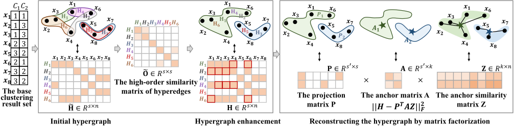
To address these challenges, we propose a novel method named dynamic anchor-based ensemble clustering via hypergraph reconstruction (YACHT). Specifically, as shown in Figure 1, YACHT transforms the base clustering results into a hypergraph and designs a hypergraph enhancement strategy based on random walks on hyperedges to improve the reliability of the initial hypergraph. Then, YACHT reconstructs the hypergraph through matrix factorization. During the reconstruction process, both the anchor matrix and the anchor similarity matrix are incorporated into the optimization objective for dynamic learning. Moreover, a mapping matrix is introduced to filter out redundant information in the hypergraph. This helps capture a higher-quality anchor similarity matrix. Next, YACHT incorporates the hypergraph into the optimization objective and imposes a hypergraph regularizer. The regularizer constrains the hypergraph update and derives a label partition. YACHT aligns the label partition with the local consensus information extracted from the base clustering results. This alignment strategy helps constrain the hypergraph to retain local consensus information during the update process without introducing significant deviations. Finally, the final consensus results are obtained by applying the Kmeans method to the anchor similarity matrix.
The main contributions of this paper are:
- We propose a novel method named dynamic anchorbased ensemble clustering via hypergraph reconstruction (YACHT). Compared to methods based on the CA matrix, YACHT reduces the time complexity to O(n) and is more suitable for large-scale datasets.
- We introduce a hypergraph enhancement strategy to improve the reliability of the initial hypergraph. The hypergraph regularizer and local consensus information alignment term are imposed to prevent significant deviations during the hypergraph update process.
- We design an alternating optimization strategy for the objective function. The effectiveness of YACHT is demonstrated through comparisons with 17 representative clustering methods.
2 RelatedWork
2.1 Ensemble Clustering
Strehl and Ghosh [Strehl and Ghosh, 2003] conducted early research on ensemble clustering, defining ensemble clustering as the process of learning a consensus result from a set of base clustering results. Ensemble clustering alleviates the robustness and stability issues of single-clustering methods. It can be broadly divided into two categories: methods based on the quality of base clustering results and methods based on consensus function strategies. The former either selects high-quality base clustering results from the base clustering set or relies on robust clustering algorithms to generate more accurate base clustering results [Huang et al., 2023; Abbasi et al., 2019; Zhao et al., 2017]. Methods based on consensus function strategies have garnered wide attention due to their excellent performance. These include CA matrixbased methods [Tao et al., 2019; Liu et al., 2015; Xie et al., 2024] and bipartite graph-based methods. CA matrix-based methods focus on improving the quality of the CA matrix [Hao et al., 2024; Jia et al., 2024] or learning its underlying subspace to explore cluster structures [Tao et al., 2019; Tao et al., 2021]. Bipartite graph-based methods leverage the association between samples and clusters to obtain consensus partitions [Fern and Brodley, 2004]. Some of these methods adopt self-paced learning frameworks to progressively learn consensus results [Zhou et al., 2021a].
2.2 Anchor based Clustering
A large number of anchor-based clustering methods have been proposed [Liu et al., 2024; Wan et al., 2023]. The motivation for introducing anchors in clustering is to enhance the scalability of the algorithm. Anchors are representative samples selected from the data, which are then used to learn the affinity relationships among the samples. Research on anchors in ensemble clustering is still in its early stages. Representative methods include: Yang et al. performed spectral clustering based on anchors and then assigned samples to the nearest anchor clusters, significantly improving timeliness [Yang et al., 2023]. Li et al. proposed an ensemble method that reuses anchor similarity matrix and employs light-k-means [Li et al., 2023]. Zhang et al. introduced a fast k-nearest neighbor approximation method to construct similarity matrices for approximating affinity matrix [Zhang et al., 2024a]. However, a key limitation of these methods is that they used raw data features to select anchors, compromising the privacy-protecting characteristics of ensemble clustering. Huang and Liang's methods [Huang et al., 2020; Liang et al., 2020] did not incorporate data features. However, their methods either used fixed anchors or ignore local consensus information, leading to poorer performance. Unlike the methods mentioned above, our method does not introduce data features, allowing for dynamic anchor learning and fully leveraging local consensus information.
3 The ProposedMethod
This section details the YACHT method, covering the objective function, optimization, and time complexity analysis.
3.1 Constructing and Enhancing the Hypergraph
Given n samples X = {x1, x2, ..., xn} and m base clustering results Ξ = {C1, C2, ..., Cm}, where xi denotes the i-th sample. Cj = {π1 j , π2 j , ..., πsj j } represents the j-th base clustering result that partitions X into sj base clusters. πh j represents the h-th base cluster in Cj. A hypergraph G = (V, E, ˜W) can be constructed from the base clustering results, where V represents the set of nodes, each corresponding to a sample. Each hyperedge in the hyperedge set E can represent a base cluster. Therefore, the number of hyperedges is equal to the number of base clusters s = ∑mj=1 sj. As shown in Figure 1, we can construct the initial hypergraph indicator matrix ˜H. The hyperedge weight ˜W is a diagonal matrix, where the diagonal elements ˜Wii represents the weights of the i-th hyperedge. Since each hyperedge represents a base cluster, we use local entropy weights [Huang et al., 2018] to represent the weights of the hyperedges. The hyperedge weights are defined as:
where p( ˜Hi:, ˜Hj:) = | ˜Hi: ⋂ ˜Hj:| | ˜Hi: | represents the ratio of the number of intersecting samples between two hyperedges to the number of samples in i-th hyperedge. θ represents the weight decay parameter, where a smaller value indicates faster weight decay.
Due to the weaknesses of the base clustering algorithms, the reliability and stability of the initial hypergraph generated from the base clustering results are compromised [Zhou et al., 2022]. We improve the reliability of the hypergraph by introducing random walks to explore the proximity between hyperedges [Zhang et al., 2024b]. We use the Jaccard distance to define the direct similarity between hyperedges:
where Oij represents the similarity between the i-th and j-th hyperedges. NormalizingOas ˙O= D-1 o Oallows it to be interpreted as a probability transition matrix, where Do denotes the Laplacian matrix of O. Then, the high-order relationship matrix ˜O ∈ Rs×s of the hyperedges is defined as:
where ˙O(d) = ˙O(d-1)⊤ ˙O. Based on this similarity, we can improve the existing hypergraph structure. We generate the enhanced hypergraph H ∈ Rs×n as follows:
where 1 (·) is a mapping function that maps all values greater than 0 to 1, and α is the similarity threshold. As shown in Eq. (2), the hyperedges of the enhanced hypergraph H may change, resulting in new hyperedge weights W.
3.2 Reconstructing the Hypergraph with Hypergraph Regularization
After obtaining the enhanced hypergraph H, a self-expressive model is employed to capture sample affinities:
where S ∈ Rn×n denotes the similarity matrix and D is the dictionary. This form can reconstruct H, but has the following issues: (i) the similarity matrix S is n × n, and the reconstruction of H is slow, leading to lower computational efficiency; (ii) it cannot filter out the redundant information in the hypergraph. Therefore, we introduce anchor learning and a mapping matrix. The anchor points reduce the similarity matrix dimension from n × n to k × n relations, where k is the number of anchor points. This results in a smaller anchor similarity matrix Z compared to S, thereby accelerating the reconstruction process. The introduction of the mapping matrix helps filter out redundant hyperedges in the hypergraph, which aids in capturing a higher-quality anchor similarity matrix. Therefore, we obtain the following form:
where P ∈ Rs′×s is the projection matrix, Z ∈ Rk×n is the similarity matrix representing the relationship between the anchors and the samples, and A ∈ Rs′×k denotes the anchor matrix. s′ is the number of representative base clusters. The orthogonal constraints on variables P and A help learn a better similarity matrix Z [Feng et al., 2024].
Furthermore, we attempt to incorporate H into the optimization objective, as the quality of H directly impacts the reliability of Z. However, unconstrained updates inevitably lead to large errors and unreliable Z. Therefore, to learn a better hypergraph, we apply the widely used hypergraph regularizer [Gao et al., 2022; Zhang et al., 2018]. We rewrite equation (3) as:
where L = I - D-1/2 v H⊤WD-1 e HD-1/2 v is the Laplacian matrix of the hypergraph. Dv = diag(H⊤W1) denotes the node degree matrix, De = diag(1⊤H⊤) is the edge degree matrix. This regularizer not only constrains the hypergraph update but also derives a label indicator matrix F ∈ Rn×c , where c is the number of clusters. The label indicator matrix helps us align the local consensus information derived from the base clustering results. This ensures that the hypergraph preserves this information during the optimization process while avoiding significant deviations.
3.3 Aligning Local Consensus Information
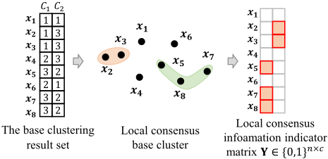
In general, local consensus information refers to results that are reflected in all base clustering results, for example, when two samples are clustered together in every base clustering perspective. Since the CA matrix captures relationships at the sample level, local consensus information can be easily applied in methods based on the CA matrix [Jia et al., 2021; Jia et al., 2024; Li et al., 2024]. To align local consensus information with the label indicator matrix F derived from the hypergraph, we also need to define a consensus base cluster S to match the size of F.
Definition 1. Let S be a set of objects. The set S is a consensus base cluster if and only if (i) ∀xi, xj ∈ S s.t. ˜H:i = ˜H:j, and (ii) the number of samples contained in the set, num(S), is at least 2 (num(S)).
Definition 1 provides the definition of consensus base cluster based on the initial hypergraph. Although both consensus base clusters and microclusters [Huang et al., 2016] require consistent sample-base cluster relationships (i.e. ˜H:i = ˜H:j), we additionally require that consensus base clusters contain more than 2 samples. This is because microclusters can include single samples, but retaining a consensus base cluster with only a single sample for alignment is meaningless. Considering the size of F, we strive to retain as much information as possible from the large number of local consensus base clusters. We first sort the number of samples in all consensus base clusters and then retain the top c consensus base clusters. Based on these c base clusters, we generate the local consensus information indicator matrix. Figure 2 shows the construction process of the local consensus information indicator matrix Y. Note that all of this is based solely on the base clustering results, without relying on any ground truth. Finally, we minimize the error between F and Y to achieve alignment. The final objective function is as follows:
3.4 Optimization
To solve Eq. (5), we employ the alternating optimization strategy [Zhong and Pun, 2022], i.e., optimizing the target variable alternately while fixing other variables.
Update P To update the variable P, other variables need to be fixed. The subproblem w.r.t. P is as follows:
We expand the Frobenius norm by the trace operation and remove terms unrelated to P, further transforming Eq. (6) into the following form:
where Q = AZH⊤. Supposing the Singular value decomposition (SVD) of Q is UQΣQV⊤Q, we can obtain the optimal solution for P as UQV⊤Q.
Update A With P, Z, H and F being fixed, the subproblem for A is as follows:
Similar to the subproblem for P, we transform the subproblem for A into the following form by expanding the Frobenius norm:
where B = PHZ⊤. Similarly, we perform the SVD decomposition B = UBΣBV⊤ B, and then obtain the optimal solution for the variable A as UBV⊤ B.
Update Z With P, A, H and F being fixed, the subproblem for Z is as follows:
Eq. (9) can be solved using the augmented Lagrange multiplier (ALM) method [Bazaraa et al., 2013]. Its augmented Lagrangian function is as follows:
where J ∈ Rn×1 represents the Lagrange multiplier, µ is the penalty parameter. Next, we take the derivative of Eq. (10) and set it to zero. The variable Z can be updated by:
Update H With P, A, Z and F being fixed, the subproblem for H is as follows:
Since Dv and De are related to H, we need to first take the derivatives of Dv and De before taking the derivative of Eq. (11). Denote that D- 12 v = diag ([dv1 , ..., dvn ]) and D-1 e = diag ([de1 , ..., den ]). We can get:
Algorithm 1 Obatain label indicator matrix F
Input: Matrix G, Y.
Output: F.
- 1: Initialize an orthogonal matrix F satisfying FF⊤ = I.
- 2: while not converged do
- 3: Update Q′ by Q′ =GF+2Y.
- 4: Calculate the SVD of Q′ =UQ′ΣQ′V⊤Q′ .
- 5: Update F by F =UQ′V⊤Q′ .
- 6: end while
where δ is the Kronecker delta, i.e., δiq = 1 if i = q and δiq = 0 otherwise. Let the subproblem for Eq. (11) be denoted as Q (H). The derivative w.r.t. H can be written as:
where J is a matrix where all elements are 1. Setting the derivative ∇Q to 0 and then solving is quite difficult, so we use the projected gradient method to optimize the variable H [Gao et al., 2022]. H is updated as follows:
where α is the learning rate, and P is the projection onto the feasible set {H|1 ≥ H ≥ 0}. P is defined as follows:
Update F With P, A, Z and H being fixed, the subproblem for F is as follows:
where G = D-1/2 v H⊤WD-1 e HD-1/2 v . Inspired by [Zhuge et al., 2019], we solve for variable F using Algorithm 1 and obtain its closed-form solution.
Update J and µ The Lagrange multipliers and penalty parameters in the ALM method are updated as follows:
where ρ > 0 is a user-defined constant, and µmax represents the maximum value of µ. The overall process of the algorithm is summarized in Algorithm 2.
3.5 Complexity Analysis
In YACHT, the time complexity is mainly driven by the hypergraph enhancement strategy and the updates of several variables. The hypergraph enhancement strategy involves random walks on the hyperedges and matrix multiplication, with a time complexity of O(s3 ). For variable P, its update
Algorithm 2 YACHT
Input: m base clustering results, c, k and α.
Output: Consensus result s.
- 1: Initialize P, A, Z, and J. Construct the initial hypergraph ˜H and obtain the enhanced hypergraph H.
- 2: while not converged do
- 3: Update P by solving Eq. (7).
- 4: Update A by solving Eq. (8).
- 5: Update Z by solving Eq. (9).
- 6: Update H by solving Eq. (11).
- 7: Update F by Algorithm 1.
- 8: Update J and µ by Eq. (15).
- 9: end while
- 10: Obtain the left singular vector U by performing SVD on Z. Perform k-means method on U to obtain s.
| No. | Dataset | Instance | Feature | Class |
|---|---|---|---|---|
| D1 | Tr12 | 313 | 5804 | 8 |
| D2 | Cars | 392 | 8 | 3 |
| D3 | IS | 2310 | 19 | 7 |
| D4 | Segment | 2310 | 18 | 7 |
| D5 | MnistData 05 | 3495 | 653 | 10 |
| D6 | MnistData 10 | 6996 | 688 | 10 |
| D7 | COIL100 | 7200 | 1024 | 100 |
| D8 | FashionMNIST | 60000 | 784 | 10 |
| D9 | KannadaMNIST | 60000 | 784 | 10 |
| D10 | EMNIST | 280000 | 784 | 10 |
process involves SVD decomposition and matrix multiplication, resulting in a time complexity of O(s′ s2 + s′n(k + s)). For variable A, its time complexity is O(s′k2 + s′n(k + s)). For variable Z, it involves matrix inversion, resulting in a time complexity of O(k3 ). For variable H, we use the projected gradient method for optimization. In each iteration, the time complexity of the computation can be reduced to O(n) by appropriately applying the associative law of matrix multiplication. Similarly, for variable F, by adjusting the order of matrix multiplication, its computational complexity can be controlled within O(c2n). According to [Zhou et al., 2022], the number of base clusters is much smaller than the number of samples, so we have n >> s, n >> k, and n >> s′ . Overall, the total time complexity of YACHT is linearly related to the number of samples, O(n).
4 Experiment
4.1 Experimental Setup
We conduct extensive experiments on 10 real datasets. Characteristics of these datasets are provided in Table 1. Some methods [Zhou et al., 2019; Tao et al., 2019] provide relevant base clustering results, which we use directly for convenience. For the other datasets 1 , we randomly run the K-means method 100 times to generate the base clustering result set.
1 http://archive.ics.uci.edu/datasets
| Dataset | D1 | D2 | D3 | D4 | D5 | D6 | D7 | D8 | D9 | D10 |
|---|---|---|---|---|---|---|---|---|---|---|
| ACC | ||||||||||
| Base clusterings (average) | 45.2±5.7 | 23.0±8.6 | 38.7±13.6 | 59.9±6.5 | 53.9±3.5 | 53.6±3.4 | 44.2±1.9 | 52.3±4.4 | 69.8±5.3 | 55.6±0.4 |
| Base clusterings (best) | 63.6 | 44.9 | 66.9 | 70.5 | 62.6 | 62.7 | 49.2 | 61.4 | 80.9 | 63.3 |
| ECCMS [TNNLS, 2024] | 54.2±3.1 | 52.6±5.9 | 65.3±2.5 | 62.0±0.7 | 58.1±0.7 | 54.9±1.8 | 44.1±1.2 | N/A | N/A | N/A |
| CEAM [TKDE, 2024] | 55.7±3.2 | 44.6±5.2 | 64.0±3.3 | 62.1±1.8 | 54.7±1.2 | 55.7±1.8 | 49.8±1.0 | N/A | N/A | N/A |
| SPCE [TNNLS, 2021] | 46.0±5.2 | 56.1±5.7 | 61.0±1.8 | 63.1±2.6 | 54.4±2.5 | 55.0±3.5 | 48.8±0.9 | N/A | N/A | N/A |
| CESHL [Inf. Fusion, 2022] | 49.2±3.3 | 51.4±1.0 | 66.2±3.1 | 64.5±6.2 | 57.4±1.8 | 57.0±0.5 | 30.8±4.2 | N/A | N/A | N/A |
| DREC [Neuro., 2019] | 52.7±4.7 | 48.4±6.6 | 65.1±2.8 | 58.1±5.6 | 51.1±5.4 | 55.8±2.3 | 42.6±2.5 | 49.7±3.7 | 67.1±4.9 | 52.4±2.7 |
| TRCE [AAAI, 2021] | 52.8±2.9 | 63.5±2.0 | 64.5±2.2 | 64.2±6.7 | 53.2±0.6 | 55.5±3.0 | 49.8±0.9 | N/A | N/A | N/A |
| LWEA [TCYB, 2018] | 57.4±10.8 | 53.3±7.6 | 65.7±2.6 | 63.4±3.0 | 58.0±1.6 | 48.3±0.6 | 43.4±1.4 | 51.5±2.0 | 73.2±2.5 | N/A |
| LWGP [TCYB, 2018] | 57.6±5.8 | 54.6±5.2 | 65.6±2.1 | 61.7±0.3 | 55.5±2.1 | 48.5±1.3 | 48.9±1.2 | 51.6±3.6 | 71.7±3.6 | 57.3±2.4 |
| ECPCS-HC [TSMC, 2021] | 45.3±2.9 | 49.5±4.0 | 63.8±3.1 | 62.1±0.7 | 53.0±3.6 | 52.7±1.5 | 41.4±1.1 | 51.6±2.6 | 60.9±4.1 | N/A |
| ECPCS-MC [TSMC, 2021] | 48.6±2.9 | 49.9±1.8 | 64.2±3.0 | 60.1±7.1 | 52.6±0.4 | 49.7±0.7 | 48.6±1.1 | 51.2±3.7 | 71.8±3.2 | 57.8±2.1 |
| U-SENC [TKDE, 2020] | 55.5±2.5 | 48.7±1.9 | 66.3±2.6 | 62.6±7.5 | 53.6±1.8 | 53.9±2.1 | 51.2±1.6 | 51.8±3.7 | 73.1±3.6 | 58.3±0.8 |
| SEC [KDD, 2015] | 43.9±7.6 | 49.5±8.8 | 49.2±9.1 | 56.4±5.0 | 51.2±6.0 | 48.4±3.8 | 44.3±1.5 | 45.5±5.2 | 57.9±7.5 | 53.0±4.8 |
| PTA-AL [TKDE, 2016] | 57.8±6.3 | 53.7±3.5 | 62.3±2.2 | 61.4±4.4 | 54.4±2.0 | 48.9±1.1 | 35.5±1.5 | 51.5±3.6 | 75.3±3.3 | 56.5±2.8 |
| PTA-CL [TKDE, 2016] PTGP [TKDE, 2016] | 56.8±5.0 | 47.1±7.1 | 66.2±5.5 67.0±5.5 | 62.1±4.0 | 56.2±2.9 63.8±4.8 55.4±2.0 | 49.5±0.8 49.4±0.8 | 34.5±1.5 34.5±1.2 | 52.3±3.2 52.0±2.5 | 76.3±3.8 | 56.8±4.3 55.9±3.5 |
| 57.3±5.1 | 52.1±5.0 | 64.0±4.3 | 52.9±1.7 | 75.7±3.8 | ||||||
| AWMVC [AAAI, 2023] SMVAGC-SF [TIP, 2024] | 54.9±4.5 55.7±4.2 | 47.0±6.6 47.7±6.2 | 51.2±5.9 51.6±9.0 | 64.1±6.0 | 51.1±1.8 51.8±1.8 | 53.7±3.1 | 50.3±0.8 49.9±1.2 | 50.0±4.0 51.8±2.6 | 72.2±4.3 73.2±4.4 | 56.9±2.8 57.1±4.3 |
| YACHT | 62.5±1.3 | 58.0±8.9 | 71.6±6.5 | 68.3±1.9 | 58.7±1.0 | 57.5±1.1 | 53.8±1.6 | 55.3±3.0 | 76.8±2.5 | 60.9±4.1 |
| ARI | ||||||||||
| Base clusterings (average) Base clusterings (best) | 21.8±8.4 44.1 | 3.8±2.2 9.2 | 34.4±11.1 56.7 | 47.1±4.3 54.5 | 36.8±2.3 43.1 | 36.6±2.3 43.3 | 39.3±1.8 43.7 | 36.2±2.0 41.1 | 57.8±3.7 65.7 | 38.0±2.9 42.2 |
| ECCMS [TNNLS, 2024] | 27.2±3.2 | 10.6±9.8 | 53.8±2.5 | 49.3±1.1 | 39.7±0.9 | 39.5±1.4 | 37.6±0.7 | N/A | N/A | N/A |
| CEAM [TKDE, 2024] | 32.5±4.5 | 6.2±7.6 | 48.4±4.9 | 48.9±0.9 | 35.9±3.5 | 36.6±2.1 | 46.0±0.7 | N/A | N/A | N/A |
| SPCE [TNNLS, 2021] | 27.2±5.3 | 9.6±7.6 | 46.9±4.7 | 50.8±1.8 | 38.1±0.7 | 38.9±1.0 | 47.6±1.3 | N/A | N/A | N/A |
| CESHL [Inf. Fusion, 2022] | 19.2±3.5 | 13.0±2.7 | 52.5±4.5 | 50.1±4.1 | 39.0±0.9 | 38.9±0.7 | 13.9±7.5 | N/A | N/A | N/A |
| DREC [Neuro., 2019] | 26.1±4.5 | 6.6±7.4 | 52.4±2.1 | 45.3±5.4 | 34.6±3.8 | 38.1±1.4 | 34.1±5.2 | 34.7±2.2 | 54.5±4.5 | 34.5±2.3 |
| TRCE [AAAI, 2021] | 22.8±4.7 | 18.6±6.9 | 52.0±2.0 | 49.7±4.9 | 36.8±0.5 | 37.5±1.7 | 41.5±1.3 | N/A | N/A | N/A |
| LWEA [TCYB, 2018] | 35.8±15.1 | 12.1±8.0 | 52.9±3.2 | 50.1±2.1 | 39.4±0.6 | 39.3±0.8 | 37.9±0.7 | 37.5±1.2 | 59.5±1.7 | N/A |
| LWGP [TCYB, 2018] | 31.3±12.5 | 13.5±1.0 | 54.4±1.8 | 49.7±0.8 | 38.4±1.2 | 37.2±1.6 | 42.1±1.1 | 36.7±1.5 | 58.8±2.4 | 40.2±2.0 |
| ECPCS-HC [TSMC, 2021] | 14.6±1.8 | 9.0±7.6 | 51.9±2.4 | 51.2±0.8 | 38.1±1.7 | 39.4±1.1 | 35.3±0.8 | 34.5±2.8 | 52.4±2.6 | N/A |
| ECPCS-MC [TSMC, 2021] | 18.9±3.0 | 12.5±2.4 | 53.1±2.0 | 47.0±4.5 | 36.4±0.3 | 37.2±1.3 | 42.1±0.9 | 36.3±1.8 | 58.7±2.0 | 40.6±1.9 |
| U-SENC [TKDE, 2020] | 30.2±4.0 | 12.0±2.1 | 51.6±2.1 | 48.9±4.9 | 36.9±0.9 | 37.1±1.1 | 46.0±1.0 | 36.8±2.0 | 59.8±2.6 | 41.1±0.7 |
| SEC [KDD, 2015] | 15.2±6.9 | 2.5±15.5 | 30.2±13.0 | 41.3±5.7 | 33.1±5.8 | 30.1±4.3 | 35.0±4.0 | 29.1±6.5 | 43.0±8.8 | 34.6±4.5 |
| PTA-AL [TKDE, 2016] | 30.2±7.0 | 16.4±4.1 | 49.3±3.3 | 50.8±2.1 | 37.6±1.0 | 37.8±1.6 | 31.8±1.6 | 36.5±2.0 | 61.2±2.4 | 38.0±3.1 |
| PTA-CL [TKDE, 2016] | 30.1±6.2 | 12.0±5.1 | 52.0±4.3 | 51.7±1.4 | 38.7±1.4 | 38.5±1.3 | 31.1±1.4 | 37.6±1.7 | 61.9±2.8 | 39.1±2.7 |
| PTGP [TKDE, 2016] | 29.9±6.4 | 14.3±3.7 | 54.6±3.6 | 51.9±1.9 | 38.2±1.0 | 38.6±1.6 | 31.8±0.9 | 37.1±1.5 | 61.6±2.8 | 38.7±3.1 |
| AWMVC [AAAI, 2023] | 32.5±3.2 | 8.2±7.2 | 31.7±7.8 | 50.3±5.6 | 33.0±2.0 | 35.1±2.0 | 44.7±1.1 | 33.9±1.8 | 57.5±3.5 | 38.5±2.9 |
| SMVAGC-SF [TIP, 2024] | 33.0±4.6 | 10.3±6.4 | 33.0±9.7 | 50.3±3.9 | 33.7±1.5 | 35.6±2.5 | 44.1±1.0 | 34.4±2.8 | 58.1±3.9 | 39.6±3.4 |
| YACHT | 41.1±4.3 | 23.1±13.5 | 54.7±5.8 | 52.6±1.8 | 41.5±0.6 | 40.9±1.1 | 49.1±0.9 | 38.4±2.3 | 62.0±3.2 | 43.0±3.0 |
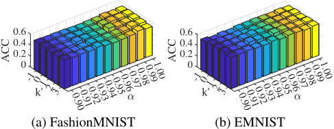
Following many ensemble methods, we set the ensemble size to 20 and conduct 10 repeated experiments with different base clustering combinations, reporting the mean and standard deviation. All compared methods use the same combination of base clustering. In YACHT, we set the hyperedge weight parameter θ = 0.4 and the maximum order of hyperedge random walks d = 20. We set the hyperparameters as follows: the number of anchors k = k′+c, where k′ ∈ {-1, 0, 1, 2, 3};
and the similarity threshold α ∈ [0.9 : 0.01 : 1]. All methods are evaluated using two popular clustering metrics: Accuracy (ACC), and Adjusted Rand Index (ARI). We use 17 representative methods, including state-of-the-art (SOTA) ensemble methods, fast ensemble methods and anchor-based clustering methods. · SOTA ensemble methods: ECCMS [Jia et al., 2024], CEAM [Zhou et al., 2024], SPCE [Zhou et al., 2021b], CESHL [Zhou et al., 2022], TRCE [Zhou et al., 2021c], DREC [Zhou et al., 2019], ECPCS-HC/MC [Huang et al., 2021]. · Fast ensemble methods: LWEA/LWGP [Huang et al., 2018], U-SENC [Huang et al., 2020], SEC [Liu et al., 2015], PTA-AL/CL [Huang et al., 2016], PTGP [Huang et al., 2016]. · Anchor-based clustering methods: AWMVC [Wan et al., 2023], SMVAGC-SF [Wang et al., 2024].
4.2 Experimental Results
Table 2 presents the experimental results on two metrics. 'N/A' indicates excessive runtime or insufficient memory. From the experimental results, we have the following observations: (i) YACHT outperforms the average results of base clustering on all metrics across all datasets, demonstrating the effectiveness of integrating multiple base clustering results. (ii) YACHT demonstrates strong performance advantages across various datasets of different sizes, highlighting the method's excellent scalability. Particularly in terms of the ARI metric, YACHT outperforms all comparison methods across all datasets. (iii) Overall, fast ensemble methods generally do not outperform SOTA ensemble methods on most datasets. However, SOTA methods are often limited by the size of the dataset and may fail to produce results. (iv) YACHT outperforms the hypergraph method CESHL across all metrics, validating the effectiveness of using anchors to reconstruct the hypergraph.
4.3 Parameter Study and Time Comparison
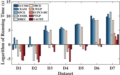
Figure 3 shows the impact of different parameter combinations on the accuracy of the YACHT method. We observe that, on large-scale datasets, the YACHT method is not highly sensitive to parameter combinations, indicating that YACHT exhibits good robustness. For large-scale datasets (FashionMNIST, EMNIST), we select no more than twenty anchor points to reconstruct the hypergraph, achieving the highest clustering accuracy, which validates the effectiveness of the reconstruction. Additionally, the parameter α has some impact on the accuracy of the YACHT method, indicating that although H is incorporated into the optimization objective, the initial values still affect the clustering accuracy. This also suggests that the hypergraph enhancement strategy can adjust the hypergraph structure through a threshold, providing a better initial value for the optimization method. Figure 4 shows a comparison of the running time across different methods. Although the YACHT method is not the fastest ensemble clustering method, it is the first to introduce a dynamic anchor learning strategy compared to existing fixed-anchor ensemble methods. Dynamic anchor learning significantly improves Dataset accuracy, but updating the anchors inevitably requires more time. In practical applications, accepting a bit of additional runtime is reasonable in order to achieve higher accuracy.
| Dataset | Metric | w/o H-Re | w/o H-r | w/o H-e | YACHT |
|---|---|---|---|---|---|
| D3 | ACC | 0.616 | 0.700 | 0.681 | 0.716 |
| ARI | 0.468 | 0.538 | 0.506 | 0.547 | |
| D9 | ACC | 0.719 | 0.755 | 0.768 | 0.768 |
| ARI | 0.586 | 0.610 | 0.620 | 0.620 |
Table 3: Ablation study results.
4.4 Ablation Study
Table 3 shows the results of the ablation versions of the YACHT method. 'w/o H-Re' indicates the version without hypergraph reconstruction, where k-means is applied directly on the hypergraph. 'w/o H-r' indicates the version using hypergraph reconstruction only, without hypergraph update and regularization. 'w/o H-e' refers to the version without the hypergraph enhancement strategy. We observe that the clustering accuracy significantly decreases without hypergraph reconstruction, which suggests that reconstruction helps remove erroneous information, improving clustering accuracy. Overall, the absence of the hypergraph enhancement strategy and the lack of hypergraph regularizer both lead to a decrease in clustering accuracy. This demonstrates the effectiveness of hypergraph reconstruction and the hypergraph regularizer in the YACHT method.
5 Conclusion
This paper proposes a dynamic anchor-based learning and hypergraph reconstruction ensemble clustering method, YACHT. YACHT transforms the base clustering results into a hypergraph and designs a hypergraph enhancement strategy to improve its reliability. Unlike other methods, YACHT learns a high-quality anchor similarity matrix through hypergraph reconstruction. Additionally, it constructs a more reliable hypergraph and constrains its update using a local consensus alignment term and hypergraph regularization. Experiments on real datasets validate the effectiveness of YACHT. Although YACHT is not the fastest ensemble method, its accuracy significantly outperforms existing SOTA methods.
Acknowledgments
This work was supported in part by the National Natural Science Foundation of China (62472294) and Grant 2024ZD0607700.
@inproceedings{ijcai2025p750,
  title     = {Dynamic Anchor-based Ensemble Clustering via Hypergraph Reconstruction},
  author    = {Xu, Jiaxuan and Duan, Lei and Wang, Xinye and Du, Liang},
  booktitle = {Proceedings of the Thirty-Fourth International Joint Conference on
               Artificial Intelligence, {IJCAI-25}},
  publisher = {International Joint Conferences on Artificial Intelligence Organization},
  editor    = {James Kwok},
  pages     = {6740--6748},
  year      = {2025},
  month     = {8},
  note      = {Main Track},
  doi       = {10.24963/ijcai.2025/750},
  url       = {https://doi.org/10.24963/ijcai.2025/750},
}
TY - CPAPER TI - Dynamic Anchor-based Ensemble Clustering via Hypergraph Reconstruction AU - Xu, Jiaxuan AU - Duan, Lei AU - Wang, Xinye AU - Du, Liang T2 - Proceedings of the Thirty-Fourth International Joint Conference on Artificial Intelligence, IJCAI-25 PB - International Joint Conferences on Artificial Intelligence Organization PY - 2025 SP - 6740 EP - 6748 DO - 10.24963/ijcai.2025/750 UR - https://doi.org/10.24963/ijcai.2025/750 ER -Copied
Machine-readable versions of this paper, for tools and AI agents:





