
PerfSeer: An Efficient and Accurate Deep Learning Models Performance Predictor
Proceedings of the Thirty-Fourth International Joint Conference on Artificial Intelligence. Main Track. Pages 7128-7136.
https://doi.org/10.24963/ijcai.2025/793
Keywords
- Machine Learning: ML: Applications
Abstract
Predicting the performance of deep learning (DL) models, such as execution time and resource utilization, is crucial for Neural Architecture Search (NAS), DL cluster schedulers, and other technologies that advance deep learning. The representation of a model is the foundation for its performance prediction. However, existing methods cannot comprehensively represent diverse model configurations, resulting in unsatisfactory accuracy. To address this, we represent a model as a graph that includes the topology, along with node, edge, and global features, all of which are crucial for effectively capturing the performance of the model. Based on this representation, we propose PerfSeer, a novel predictor that uses a Graph Neural Network (GNN)-based performance prediction model, SeerNet. SeerNet fully leverages the topology and various features, while incorporating optimizations such as Synergistic Max-Mean aggregation (SynMM) and Global-Node Perspective Boost (GNPB) to more effectively capture the critical performance information, enabling it to predict the performance of models accurately. Furthermore, SeerNet can be extended to SeerNet-Multi by using Project Conflicting Gradients (PCGrad), enabling efficient simultaneous prediction of multiple performance metrics without significantly affecting accuracy. We constructed a dataset containing performance metrics for 53k+ model configurations, including execution time, memory usage, and Streaming Multiprocessor (SM) utilization during both training and inference. The evaluation results show that PerfSeer outperforms nn-Meter, Brp-NAS, and DIPPM.
- [Banbury et al., 2021] Colby Banbury, Chuteng Zhou, Igor Fedorov, Ramon Matas Navarro, Urmish Thakker, Dibakar Gope, Vijay Janapa Reddi, Matthew Mattina, and Paul N. Whatmough. Micronets: Neural network archi- tectures for deploying tinyml applications on commodity microcontrollers, 2021.
- [Battaglia et al., 2018] Peter W Battaglia, Jessica B Ham- rick, Victor Bapst, Alvaro Sanchez-Gonzalez, Vinicius Zambaldi, Mateusz Malinowski, Andrea Tacchetti, David Raposo, Adam Santoro, Ryan Faulkner, et al. Relational inductive biases, deep learning, and graph networks. arXiv preprint arXiv:1806.01261, 2018.
- [Chai et al., 2023] Yuji Chai, Devashree Tripathy, Chuteng Zhou, Dibakar Gope, Igor Fedorov, Ramon Matas, David Brooks, Gu-Yeon Wei, and Paul Whatmough. Perfsage: Generalized inference performance predictor for arbitrary deep learning models on edge devices. arXiv preprint arXiv:2301.10999, 2023.
- [Chen and Guestrin, 2016] Tianqi Chen and Carlos Guestrin. Xgboost: A scalable tree boosting system. In Proceedings of the 22nd acm sigkdd international conference on knowl- edge discovery and data mining, pages 785-794, 2016.
- [Dong and Yang, 2020] Xuanyi Dong and Yi Yang. Nas- bench-201: Extending the scope of reproducible neural ar- chitecture search. In International Conference on Learn- ing Representations, 2020.
- [Dudziak et al., 2020] Lukasz Dudziak, Thomas Chau, Mo- hamed Abdelfattah, Royson Lee, Hyeji Kim, and Nicholas Lane. Brp-nas: Prediction-based nas using gcns. Advances in Neural Information Processing Systems, 33:10480- 10490, 2020.
- [Eriksson et al., 2021] David Eriksson, Pierce I-Jen Chuang, Samuel Daulton, Peng Xia, Akshat Shrivastava, Arun Babu, Shicong Zhao, Ahmed Aly, Ganesh Venkatesh, and Maximilian Balandat. Latency-aware neural architecture search with multi-objective bayesian optimization, 2021.
- [Fedorov et al., 2019] Igor Fedorov, Ryan P. Adams, Matthew Mattina, and Paul N. Whatmough. Sparse: Sparse architecture search for cnns on resource- constrained microcontrollers, 2019.
- [Gao et al., 2023] Yanjie Gao, Xianyu Gu, Hongyu Zhang, Haoxiang Lin, and Mao Yang. Runtime performance pre- diction for deep learning models with graph neural net- work. In 2023 IEEE/ACM 45th International Conference on Software Engineering: Software Engineering in Prac- tice (ICSE-SEIP), pages 368-380. IEEE, 2023.
- [Gilmer et al., 2017] Justin Gilmer, Samuel S. Schoenholz, Patrick F. Riley, Oriol Vinyals, and George E. Dahl. Neural message passing for quantum chemistry. In Proceedings of the 34th International Conference on Machine Learning - Volume 70, ICML'17, page 1263-1272. JMLR.org, 2017.
- [Gu et al., 2021] Rong Gu, Yuquan Chen, Shuai Liu, Haipeng Dai, Guihai Chen, Kai Zhang, Yang Che, and Yi- hua Huang. Liquid: Intelligent resource estimation and network-efficient scheduling for deep learning jobs on dis- tributed gpu clusters. IEEE Transactions on Parallel and Distributed Systems, 33(11):2808-2820, 2021.
- [Hamilton et al., 2017] Will Hamilton, Zhitao Ying, and Jure Leskovec. Inductive representation learning on large graphs. Advances in Neural Information Processing Sys- tems, 30, 2017.
- [Haykin, 1998] Simon Haykin. Neural networks: a compre- hensive foundation. Prentice Hall PTR, 1998.
- [He et al., 2016] Kaiming He, Xiangyu Zhang, Shaoqing Ren, and Jian Sun. Deep residual learning for image recog- nition. In Proceedings of the IEEE conference on computer vision and pattern recognition, pages 770-778, 2016.
- [Hopfield, 1982] John J Hopfield. Neural networks and physical systems with emergent collective computational abilities. Proceedings of the national academy of sciences, 79(8):2554-2558, 1982.
- [Howard et al., 2017] Andrew G Howard, Menglong Zhu, Bo Chen, Dmitry Kalenichenko, Weijun Wang, Tobias Weyand, Marco Andreetto, and Hartwig Adam. Mo- bilenets: Efficient convolutional neural networks for mo- bile vision applications. arXiv preprint arXiv:1704.04861, 2017.
- [Huang et al., 2017] Gao Huang, Zhuang Liu, Laurens Van Der Maaten, and Kilian Q Weinberger. Densely connected convolutional networks. In Proceedings of the IEEE con- ference on computer vision and pattern recognition, pages 4700-4708, 2017.
- [Justus et al., 2018] Daniel Justus, John Brennan, Stephen Bonner, and Andrew Stephen McGough. Predicting the computational cost of deep learning models. In 2018 IEEE international conference on big data (Big Data), pages 3873-3882. IEEE, 2018.
- [Kipf and Welling, 2017] Thomas N. Kipf and Max Welling. Semi-supervised classification with graph convolutional networks, 2017.
- [Krizhevsky et al., 2012] Alex Krizhevsky, Ilya Sutskever, and Geoffrey E Hinton. Imagenet classification with deep convolutional neural networks. Advances in Neural Infor- mation Processing Systems, 25, 2012.
- [Liaw et al., 2002] Andy Liaw, Matthew Wiener, et al. Clas- sification and regression by randomforest. R news, 2(3):18-22, 2002.
- [Panner Selvam and Brorsson, 2023] Karthick Panner Sel- vam and Mats Brorsson. Dippm: A deep learning infer- ence performance predictive model using graph neural net- works. In European Conference on Parallel Processing, pages 3-16, 2023.
- [Simonyan and Zisserman, 2015] Karen Simonyan and An- drew Zisserman. Very deep convolutional networks for large-scale image recognition. In Yoshua Bengio and Yann LeCun, editors, 3rd International Conference on Learning Representations, ICLR 2015, San Diego, CA, USA, May 7-9, 2015, Conference Track Proceedings, 2015.
- [Szegedy et al., 2015] Christian Szegedy, Wei Liu, Yangqing Jia, Pierre Sermanet, Scott Reed, Dragomir Anguelov, Dumitru Erhan, Vincent Vanhoucke, and Andrew Rabi- novich. Going deeper with convolutions. In Proceedings of the IEEE conference on computer vision and pattern recognition, pages 1-9, 2015.
- [Velickovic et al., 2017] Petar Velickovic, Guillem Cucu- rull, Arantxa Casanova, Adriana Romero, Pietro Lio, Yoshua Bengio, et al. Graph attention networks. stat, 1050(20):10-48550, 2017.
- [Xie et al., 2017] Saining Xie, Ross Girshick, Piotr Dollár, Zhuowen Tu, and Kaiming He. Aggregated residual trans- formations for deep neural networks. In Proceedings of the IEEE conference on computer vision and pattern recogni- tion, pages 1492-1500, 2017.
- [Yeung et al., 2021] Gingfung Yeung, Damian Borowiec, Renyu Yang, Adrian Friday, Richard Harper, and Peter Garraghan. Horus: Interference-aware and prediction- based scheduling in deep learning systems. IEEE Transac- tions on Parallel and Distributed Systems, 33(1):88-100, 2021.
- [Yu et al., 2020] Tianhe Yu, Saurabh Kumar, Abhishek Gupta, Sergey Levine, Karol Hausman, and Chelsea Finn. Gradient surgery for multi-task learning. In Proceedings of the 34th International Conference on Neural Informa- tion Processing Systems, NIPS '20, page 13, Red Hook, NY, USA, 2020.
- [Curran Associates Inc. Zhang et al., 2021] Li Lyna Zhang, Shihao Han, Jianyu Wei, Ningxin Zheng, Ting Cao, Yuqing Yang, and Yunxin Liu. Nn-meter: Towards accurate latency prediction of deep-learning model inference on diverse edge devices. In Proceedings of the 19th Annual International Conference on Mobile Systems, Applications, and Services, pages 81- 93, 2021.
References were extracted automatically from the PDF and may contain errors.
Full text extracted automatically from the PDF; figures, tables and equations may differ. The PDF is the version of record.
1 Introduction
Deep learning (DL) has achieved significant success across various fields [Hopfield, 1982; Krizhevsky et al., 2012]. Understanding the performance of models (e.g., execution time and resource utilization) is crucial for technologies such as Neural Architecture Search (NAS) and DL cluster schedulers, which drive the advancement of deep learning. NAS relies on performance metrics like execution time [Dudziak et al., 2020; Eriksson et al., 2021] and memory usage [Fedorov et al., 2019; Banbury et al., 2021] to design efficient models that meet real-time requirements and hardware constraints. Similarly, efficient DL cluster schedulers use these metrics to reduce job completion time and improve accelerator utilization [Gu et al., 2021; Yeung et al., 2021].
* Corresponding authors.
Acquiring performance metrics through online profiling is both time-consuming and costly. Consequently, various predictors have been proposed to predict the model performance, generally categorized into three main methods. The first method [Gu et al., 2021; Yeung et al., 2021] treats the model as a whole, representing it with global features like floating point operations (FLOPs). These features are then used in a basic model, such as Multi-Layer Perceptron (MLP) [Haykin, 1998], to predict the performance. The second method [Justus et al., 2018; Zhang et al., 2021] divides the model into multiple parts (e.g., operations or units), each represented by specific features. These features are then fed into a similar basic model to predict the performance of each part, which is aggregated to estimate the overall performance. The third method [Dudziak et al., 2020; Gao et al., 2023; Panner Selvam and Brorsson, 2023; Chai et al., 2023] treats the model as a computational graph, represented by its topology and node features. These are then fed into a GNN-based model. This approach enables more accurate predictions by learning the performance of each operation and its interdependencies. Overall, performance predictors use machinereadable data to represent models and then feed this data into prediction models to predict the performance.
However, the model representation in these predictors is not comprehensive enough, resulting in the loss of important information related to model performance, leading to suboptimal prediction accuracy. Specifically, node, edge, and global features are all crucial for a model. Node features capture the characteristics of each operation. Edge features describe the data flow and dependencies between operations. Global features provide a view of the overall structure and complexity of the model. Existing predictors have not selected, constructed, and leveraged these features effectively.
We propose PerfSeer, a novel predictor that can comprehensively represent the model and fully leverage this representation to accurately predict the performance of models.
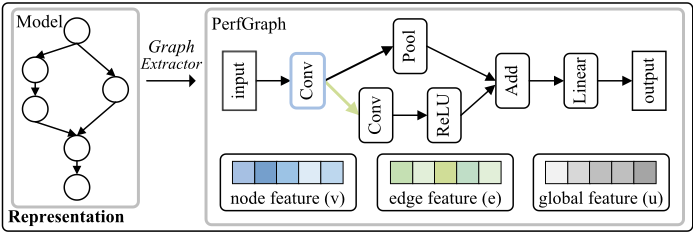
Initially, PerfSeer uses Graph Extractor to parse the computational graph of a model and generate a performance graph (PerfGraph), which can represent the model performance. This graph, in addition to the topology, also contains the node, edge, and global features, all of which improve the performance prediction accuracy. Notably, we construct several unique and effective features, such as arithmetic intensity and statistics of computation and memory access, which are not used by any previous predictors and have been empirically proven to enhance prediction accuracy noticeably.
Subsequently, the PerfGraph is fed into our proposed prediction model, SeerNet, to predict the performance. SeerNet, inspired by [Battaglia et al., 2018], enables each feature to update its own representation by utilizing both its own features and aggregated information from other features. This allows SeerNet to not only learn the topology but also fully leverage various features, providing a comprehensive understanding of the model. Specifically, it learns computation and memory access of each operation from the node features, data flow and dependencies between operations from the edge features, and the structure and complexity of the entire model from the global features. To more effectively capture the performance information of models from these features, SeerNet proposes Synergistic Max-Mean aggregation (SynMM) and Global-Node Perspective Boost (GNPB). SynMM can better aggregate node features, generating a more comprehensive and robust model representation. GNPB enables complementary learning between the node and global features, mutually enriching their perspectives.
In addition, We propose SeerNet-Multi, a multi-metric performance prediction model designed for applications that require simultaneous consideration of multiple metrics (e.g., [Yeung et al., 2021; Gu et al., 2021]). Training and maintaining separate models for each metric is inefficient, so SeerNetMulti extends SeerNet with multiple prediction heads to predict multiple metrics simultaneously. To address conflicts in parameter updates caused by differing gradient directions across tasks, we integrate Projecting Conflicting Gradients (PCGrad) [Yu et al., 2020], ensuring high accuracy. As a result, SeerNet-Multi provides efficient and accurate multimetric predictions.
We constructed a dataset with over 53k model configurations, covering key performance metrics such as execution time, memory usage, and Streaming Multiprocessor (SM) utilization during both training and inference in Nvidia GeForce RTX 3090. The dataset spans various architectures, such as VGG [Simonyan and Zisserman, 2015], GoogLeNet [Szegedy et al., 2015], ResNe(X)t [He et al., 2016; Xie et al., 2017], MobileNet [Howard et al., 2017], and DenseNet [Huang et al., 2017]. It also includes a wide range of FLOPs, from 49M to 22T. Evaluation results show that SeerNet achieves an average Mean Absolute Percentage Error (MAPE) of 5.14%, while SeerNet-Multi achieves 7.75% MAPE, outperforming other predictors.
We summarize our key contributions as follows:
- We propose a novel performance predictor, PerfSeer. Experiments show that PerfSeer, with low deployment and usage overhead, predicts multiple performance met-
- rics accurately for models of various architectures and frameworks on different devices during training and inference, enabling broad applicability.
- We design the performance prediction models, SeerNet and SeerNet-Multi. SeerNet achieves state-of-theart prediction accuracy. It rigorously selects, novelly constructs, and fully leverages the performancerelated node, edge, and global features. Additionally, it enhances performance capture through SynMM and GNPB. SeerNet-Multi efficiently predicts multiple performance metrics without significantly affecting accuracy by mitigating gradient conflicts using PCGrad.
- We construct a performance dataset 1 . The dataset, which contains over 53k model configurations, covers key performance metrics across various architectures and FLOPs during both training and inference.
2 RelatedWork
Global Features-BasedPredictor. Liquid [Gu et al., 2021] and Horus [Yeung et al., 2021] use traditional models, such as Random Forest (RF) [Liaw et al., 2002] and XGBoost [Chen and Guestrin, 2016], to predict GPU utilization and memory usage during model training by inputting global features like batch size, FLOPs, and parameter size. However, these methods are limited as they fail to capture internal execution details, and different models can exhibit vastly different performance, even with the same global features.
Operations/Unit-Wise Predictor. Justus et al. [Justus et al., 2018] predict the execution time of training models on edge devices by predicting the execution time of each operation and aggregating them. They use hardware, operations, and specific features as inputs to an MLP. nn-Meter [Zhang et al., 2021] splits the model inference into kernels, predicting the execution time of each by feeding features like hyper-parameters, FLOPs, and input/output shapes into an RF model. This execution time is aggregated to get the total execution time. However, this approach relies on heuristic detection functions that require a deep understanding of execution details across different models and devices, which can be costly and inaccurate, leading to inaccurate predictions.
GNN-Based Predictor. BRP-NAS (Eagle) [Dudziak et al., 2020] uses a Graph Convolutional Network (GCN) [Kipf and Welling, 2017]-based model to predict execution time and accuracy for inference models, applied to NAS on NAS-Bench201 [Dong and Yang, 2020]. DNNPerf [Gao et al., 2023] uses node and edge features in a custom Graph Attention Network (GAT) [Velickovic et al., 2017]-based model to predict execution time and memory usage for training models. DIPPM [Panner Selvam and Brorsson, 2023] feeds node and global features into a Graph Sample and Aggregation (GraphSAGE) [Hamilton et al., 2017]-based model (PMGNS), which generates embeddings and uses multiple prediction heads to predict execution time, memory usage, and energy consumption for inference models. These approaches capture execution details of models by learning both the topology and features using GNN models, ensuring prediction accuracy.
1 https://github.com/upuuuuuu/PerfSeer
3 Methods
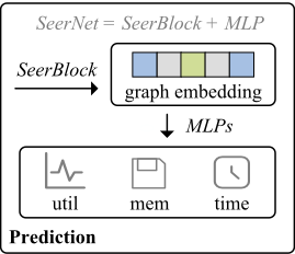
PerfSeer consists of two main parts: representation and prediction, as shown in Figure 1.
- Representation. PerfSeer uses Graph Extractor to analyze the computational graph of a model, generating a performance graph (PerfGraph) to represent the model. The PerfGraph encompasses the topology as well as the node, edge, and global features, comprehensively preserving the performance information of models (Section 3.1).
- Prediction. PerfSeer employs SeerNet and SeerNetMulti, our designed prediction models. These models effectively leverage the extracted topology and various features. They capture the critical performance information to predict metrics like execution time, memory usage, and SM utilization (Section 3.2).
Through these two parts, PerfSeer can comprehensively represent the model and fully leverage this representation to predict the model performance accurately.
3.1 Representation
We use the Graph Extractor via ONNX to generate a PerfGraph, extracting the topology and as many performancerelated features as possible to preserve and represent the performance information of models. PerfSeer is compatible with multiple DL frameworks, such as PyTorch, TensorFlow, and MXNet, unlike other predictors that support only a few.
Definition of PerfGraph
PerfGraph is defined as a 3-tuple G = (u, V, E). The u represents the global features, which are the features of the entire model. The V = {vi}i=1:N v is the set of nodes (N v is the number of nodes), where vi represents the features of node i (Node i represents operation node i in the computational graph). The E = {(ej, sj, tj)}j=1:N e is the set of edges (N e is the number of edges), where sj is the index of the source node and tj is the index of the target node, indicating a directed edge j from the source node sj to the target node tj. Edge j represents the data flow from operation sj to operation tj, where operation tj depends on operation sj, and ej represents the features of edge j.
Features of PerfGraph
The features of the PerfGraph consist of the node, edge, and global features, described as follows:
Node Features. Node features are represented as v = (vhp || vc || vm || va || vp ). || represents the concatenation, responsible for concatenating different features.
vhp represents the hyper-parameters of the node, such as the kernel size of the convolution, and serves as the fundamental representation of the node, with all other features derived from it.
- vc denotes the computation information (i.e., FLOPs) of the node, representing the computational requirements of the node.
vm represents the memory access information of the node, including the memory access cost (MAC) and the weight size. The MAC is the sum of the sizes of the input, weight, and output tensors. The features symbolize the memory access requirements of the node.
va represents arithmetic intensity, defined as the ratio of FLOPs to MAC. The features can distinguish whether the node is arithmetic-intensive or memory-intensive.
vp denotes the proportions of FLOPs, MAC, and weight size relative to the model. The features can indicate the contribution of the node to the computational and memory requirements of the model.
Edge Features. Edge features are represented as e = (esz || esp ).
- esz represents the size of the tensor delivered by the edge.
- esp represents the shape of the tensor delivered by the edge, which includes the batch size, channel, height, and width.
Global Features. Global features are represented as u = (ugp || uc || um || ua || ub ).
- ugp includes the number of nodes, edges, and density. The number of nodes (N v ) and edges (N e ) represent the counts of computations and memory accesses in the model, respectively. Density, defined as N e N v (N v -1) , reflects the interconnectedness of the nodes in the graph, indicating how densely the nodes are connected. The features provide a topological profile of the entire computational graph of the model.
uc represents FLOP statistics for all nodes in the model, including total, average, median, and maximum FLOPs. The features capture the computational characteristics of the model.
um represents memory access statistics for all nodes, such as total, average, median, and maximum values for MAC and weight size, as well as the average tensor size per edge, reflecting the memory access profile of the model.
ua denotes arithmetic intensity, the ratio of FLOPs to MAC, which helps distinguish whether the model is arithmetic-intensive or memory-intensive.
ub represents the batch size, which indicates the number of samples processed simultaneously by the model.
3.2 Prediction
SeerNet comprises a SeerBlock and an MLP-based prediction head. The PerfGraph is input into SeerBlock, which learns a graph embedding that captures the performance information from the node, edge, global features, and the topology of the computational graph. This embedding is then passed to the prediction head, a two-layer MLP with 256 hidden dimensions, to predict the performance accurately.
SeerBlock
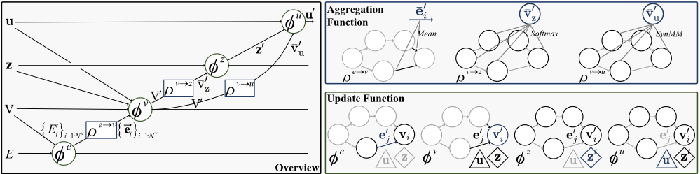
SeerBlock, inspired by [Battaglia et al., 2018], enables each feature to update its own representation by utilizing both its own features and the aggregated information from other features. The workflow of SeerBlock, shown in Figure 2, consists of four update functions (ϕ) and three aggregation functions (ρ).
Where E′ i = {(e′j , sj, tj )}tj=i, j=1:N e , V ′ = {v′i }i=1:N v , and z represents the features of the global node (see GlobalNode Perspective Boost). The details are as follows:
- ϕe is applied to per edge to compute the updated edge features, e′j . The set of resulting per-edge outputs for each node i is E′ i = {(e′j , sj , tj )}tj=i, j=1:N e .
- ρe→v is applied to E′ i to aggregate the updated edge features of edges projecting to node i into ¯e′i , which will be used in the node update in the next step.
- ϕv is applied to each node i to compute the updated node features, v′i . The set of resulting per-node outputs is V ′ = {v′i }i=1:N v .
- ρv→z is applied to V ′ to aggregate all updated nodes into ¯v′z , which will then be used to update the global node in the next step (see Global-Node Perspective Boost).
- ϕz is applied once per graph to compute the updated global node features, z′ .
- ρv→u is applied to V ′ to aggregate all updated nodes into ¯v′u , which will then be used to update global features in the next step (see Synergistic Max-Mean Aggregation).
- ϕu is applied once per graph to compute the updated global features, u′ . u′ is the output of the SeerBlock.
Each MLP in SeerBlock has one layer with 256 hidden dimensions, except for MLPz, which has two layers. Given the PerfGraph G = (u, V,E), SeerBlock produces the updated PerfGraph G′ = (u′ , V ′ , E′ ), and the graph embedding u′ is fed into the prediction head to predict performance.
Synergistic Max-Mean Aggregation
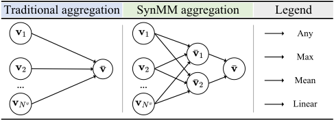
SynMM is the customized function for the node features aggregation. As shown in Figure 3, the node features are first fed into the max and mean aggregation to obtain intermediate results, ¯v1 and ¯v2. Then, linear aggregation combines these results to generate the final aggregated features, ¯v. Max aggregation extracts the most prominent features from crucial nodes, while mean aggregation captures global information and overall model characteristics. Linear aggregation consolidates the results from both max and mean aggregation, providing a more comprehensive and robust model representation.
Global-Node Perspective Boost
GNPB, inspired by [Gilmer et al., 2017], introduces a global node (z, representing its features) connected to all other nodes in the graph. It also proposes a tailored initialization strategy for z and incorporates it into the final graph embedding to enrich the global perspective of the model. The process is as follows: First, the z are initialized using softmax, aggregating the initial features of all nodes to capture global information. During the node update, each node utilizes the z to incorporate global information (Eq. 4). The z then updates itself by aggregating information from all updated nodes (Eq. 6). The global node offers a unique global perspective by aggregating information from all nodes, distinct from the global features based on the inherent characteristics of models. GNPB enables complementary learning between the node and global features, enriching both perspectives.
SeerNet-Multi
SeerNet-Multi extends SeerNet by using multiple MLP-based prediction heads to predict different performance metrics separately. In addition, PCGrad is employed to mitigate gradient conflicts among different performance metrics prediction tasks during the training of SeerNet-Multi. PCGrad works by adjusting the gradients of each task to minimize conflicts that arise when gradients point in opposing directions. The core idea is to identify conflicts by calculating the cosine similarity between the gradients of different tasks. When a conflict is detected (cosine similarity is negative, indicating opposing directions), the gradient of the task is adjusted to ensure alignment by projecting it onto the normal plane of the conflicting gradient. If no conflict is found, the gradient remains unchanged. By resolving these conflicts, PCGrad enables SeerNet-Multi to effectively predict multiple performance metrics simultaneously while maintaining accuracy.
4 Experiments
We evaluate PerfSeer by addressing the following research questions (RQs).
RQ1: How effective are the selected features and optimization components?
- RQ2: How does SeerNet compare with baseline models?
- RQ3: How effective is the multi-metric performance prediction model, SeerNet-Multi?
RQ4: What is the application scope and overhead of PerfSeer?
4.1 Evaluation Setup
Training Settings
The dataset is divided into 2:1:1 for training, validation, and testing. We use a batch size of 128 and an initial learning rate of 1e-3, halving it after five epochs without improvement, down to 1e-6. Training runs for up to 500 epochs, with Mean Squared Error (MSE) as the loss function and Adam as the optimizer.
Evaluation Metrics
To ensure consistency across metrics with varying value ranges, we use percentage errors. The metrics include MAPE, and accuracy within a relative error of x% (x%Accuracy) [Dudziak et al., 2020].
4.2 Ablation Study (RQ1)
The accuracy of the performance prediction depends on both representation and prediction. We conducted ablation studies to validate the feature selection and construction (representation) and the prediction model design (prediction).
Ablation Study of Features
From the results shown in Table 1, we observe the following: Feature Importance. Node features are more important than global features, and global features are far more important than edge features. Node features contribute the most significant gain (reducing the mean MAPE from 58.23% to 28.41%) as they directly correspond to each operation node, edge features provide incremental improvement (reducing the mean MAPE from 28.41% to 25.40%) by offering additional memory access information, and global features deliver the ultimate refinement (reducing the mean MAPE from 25.40% to 7.41%) by providing an overall representation of the model.
Feature Selection. Each group of node, edge, and global features we selected improved performance prediction accuracy, demonstrating their relevance to model performance. Additionally, we found that node categories, which are commonly used in other predictors, actually reduced accuracy, increasing the mean MAPE by 0.42% and 0.26% when onehot encoded and frequency encoded, respectively. We believe that SeerNet can infer category-related information from other semantically rich features, so we excluded node categories from our feature set.
Feature Construction. We constructed several unique and effective features. For node features, we incorporated arithmetic intensity and computation/memory access proportions, reducing the mean MAPE from 35.41% to 28.41%. For global features, we introduced graph profiles, trend statistics for computation and memory access, tensor size per edge, and arithmetic intensity, lowering the mean MAPE from 25.40% to 7.53%. These features, not used in previous predictors, significantly enhanced prediction accuracy.
Ablation Study of Components
From the results shown in Table 2, we observe the following: SynMM. Using SynMM to aggregate the node features reduces the mean MAPE from 7.41% to 6.10%. This demonstrates that SynMM combines max and mean aggregation to create a more comprehensive and robust representation, thereby enhancing prediction accuracy.
| Feature | Accuracy (MAPE[%]↓) | ||||||||||||||||||
|---|---|---|---|---|---|---|---|---|---|---|---|---|---|---|---|---|---|---|---|
| Node | Edge | Global | Training | Inference | Mean | ||||||||||||||
| Hp | CI | MAI | ArI* | Prop* | Sz | Sp | Gp* | CI* | MAI* | ArI* | Bs | Util | Mem | Time | Util | Mem | Time | (6 metrics) | |
| ✓ | ✗ | ✗ | ✗ | ✗ | ✗ | ✗ | ✗ | ✗ | ✗ | ✗ | ✗ | 71.33 | 49.56 | 54.29 | 57.04 | 24.69 | 92.49 | 58.23 | |
| ✓ | ✓ | ✗ | ✗ | ✗ | ✗ | ✗ | ✗ | ✗ | ✗ | ✗ | ✗ | 73.87 | 63.58 | 41.19 | 57.15 | 30.73 | 54.07 | 53.43 | |
| ✓ | ✓ | ✓ | ✗ | ✗ | ✗ | ✗ | ✗ | ✗ | ✗ | ✗ | ✗ | 53.71 | 37.01 | 25.98 | 46.03 | 11.45 | 38.29 | 35.41 | |
| ✓ | ✓ | ✓ | ✓ | ✗ | ✗ | ✗ | ✗ | ✗ | ✗ | ✗ | ✗ | 37.20 | 36.81 | 23.94 | 38.57 | 11.67 | 36.52 | 30.79 | |
| ✓ | ✓ | ✓ | ✓ | ✓ | ✗ | ✗ | ✗ | ✗ | ✗ | ✗ | ✗ | 38.85 | 36.76 | 23.51 | 36.32 | 11.51 | 23.51 | 28.41 | |
| ✓ | ✓ | ✓ | ✓ | ✓ | ✓ | ✗ | ✗ | ✗ | ✗ | ✗ | ✗ | 41.24 | 25.29 | 24.05 | 37.55 | 9.28 | 23.27 | 26.78 | |
| ✓ | ✓ | ✓ | ✓ | ✓ | ✓ | ✓ | ✗ | ✗ | ✗ | ✗ | ✗ | 36.02 | 27.11 | 22.31 | 33.27 | 9.93 | 23.77 | 25.40 | |
| ✓ | ✓ | ✓ | ✓ | ✓ | ✓ | ✓ | ✓ | ✗ | ✗ | ✗ | ✗ | 7.48 | 3.83 | 9.48 | 8.32 | 6.33 | 15.22 | 8.44 | |
| ✓ | ✓ | ✓ | ✓ | ✓ | ✓ | ✓ | ✓ | ✓ | ✗ | ✗ | ✗ | 7.25 | 3.72 | 8.79 | 7.93 | 5.93 | 13.08 | 7.78 | |
| ✓ | ✓ | ✓ | ✓ | ✓ | ✓ | ✓ | ✓ | ✓ | ✓ | ✗ | ✗ | 6.22 | 3.39 | 9.51 | 6.98 | 5.51 | 14.41 | 7.67 | |
| ✓ | ✓ | ✓ | ✓ | ✓ | ✓ | ✓ | ✓ | ✓ | ✓ | ✓ | ✗ | 6.23 | 3.38 | 9.45 | 7.37 | 5.29 | 13.45 | 7.53 | |
| ✓ | ✓ | ✓ | ✓ | ✓ | ✓ | ✓ | ✓ | ✓ | ✓ | ✓ | ✓ | 6.09 | 3.32 | 9.21 | 7.57 | 5.13 | 13.15 | 7.41 | |
| Component | Accuracy(MAPE[%]↓) | |||||||
|---|---|---|---|---|---|---|---|---|
| SynMM | GNPB | Training | Inference | Mean (6 metrics) | ||||
| Util | Mem | Time | Util | Mem | Time | |||
| ✗ | ✗ | 6.09 | 3.32 | 9.21 | 7.57 | 5.13 | 13.15 | 7.41 |
| ✓ | ✗ | 6.13 | 2.54 | 7.78 | 5.80 | 3.62 | 10.70 | 6.10 |
| ✓ | ✓ | 4.94 | 2.47 | 6.71 | 4.37 | 3.46 | 8.91 | 5.14 |
GNPB. With the introduction of GNPB, the mean MAPE further decreases from 6.10% to 5.14%. This result proves that GNPB enables complementary learning between the node and global features, enriching both perspectives and further improving prediction accuracy.
4.3 Baseline Comparison (RQ2)
Baseline
We compare SeerNet with the following methods: (i) MLPNode uses an MLP to predict model performance, concatenating features from all nodes in the graph and handling variable node numbers by padding or truncating them to a fixed size. (ii) PMGNS [Panner Selvam and Brorsson, 2023] (Section 2) utilizes a single prediction head for predicting one performance metric. (iii) Eagle [Dudziak et al., 2020] (Section 2) is implemented for cell-based models, but for non-cell-based models, it uses features from PMGNS (Eagle-p) and from our PerfSeer (Eagle-s). (iv) nn-Meter [Zhang et al., 2021] (Section 2) is a kernel-based predictor.
Performance Comparison
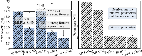
Baseline Comparison on our Dataset. Figure 4 shows that SeerNet uses the fewest parameters (1.02M) and achieves the highest accuracy, with a mean MAPE of 5.14%. In comparison, MLP-Node requires more than four times the parameters and reaches less than one-third of the accuracy (with over three times the MAPE), while PMGNS uses more than three times the parameters and achieves only about half of the accuracy. Eagle-p performs poorly, with a mean MAPE of 74.43%, because PMGNS features fail to represent the models in our comprehensive dataset effectively. Eagle-s, which adopts our proposed features, performs better but still lags behind SeerNet. Moreover, PMGNS and Eagle-s achieve higher accuracy with fewer parameters compared to MLPNode, highlighting the ability of GNN-based models to capture execution dependencies. Eagle-s outperforms Eagle-p, further confirming the effectiveness of the proposed features. Overall, SeerNet outperforms all other models, providing the best representation and prediction.
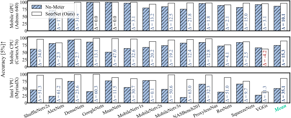
Baseline Comparison on the Dataset of nn-Meter. Figure 5 shows that SeerNet outperforms nn-Meter in average accuracy across 13 models on GPU, CPU, and VPU by 10.1%, 15.3%, and 35.1%, respectively. For models like VGG on CPU, SeerNet is slightly less accurate than nn-Meter, likely due to the simple structure of VGG. Specifically, on VPU, nn-Meter achieves 50.6% accuracy, while SeerNet reaches 85.7%, 35.1% higher. This is likely because nn-Meter fails to design effective detection functions for models on VPU.
4.4 Effectiveness of SeerNet-Multi (RQ3)
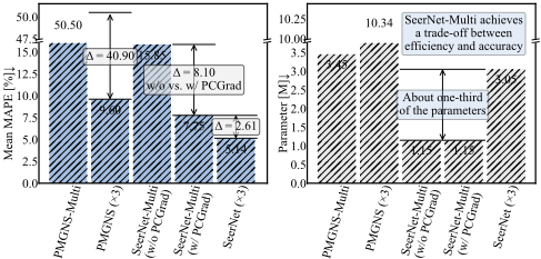
Figure 6 shows that PMGNS-Multi (with multiple prediction heads) has a poor MAPE of 50.5%, while SeerNet-Multi (without PCGrad) achieves 15.85%, indicating that predicting multiple metrics reduces accuracy. With PCGrad, SeerNetMulti achieved an MAPE of 7.75%, about half of that without PCGrad, without increasing parameters, effectively mitigating conflicting gradients and enabling efficient multi-metric prediction with minimal accuracy loss. SeerNet-Multi, with about one-third the parameters of SeerNet and a 2.61% increase in MAPE, achieves a trade-off between efficiency and accuracy, making it ideal for rapid predictions with limited resources and lower accuracy demands.
| Accuracy (MAPE[%]↓) | |||||||
|---|---|---|---|---|---|---|---|
| Dataset | Training | Inference | Mean | ||||
| scale | Util | Mem | Time | Util | Mem | Time | (6 metrics) |
| overall | 4.94 | 2.47 | 6.71 | 4.37 | 3.46 | 8.91 | 5.14 |
| 20000 | 5.49 | 2.49 | 8.58 | 5.04 | 3.83 | 13.65 | 6.51 |
| 10000 | 6.01 | 2.91 | 10.05 | 5.31 | 5.37 | 14.49 | 7.36 |
| 5000 | 7.61 | 4.24 | 10.78 | 6.32 | 4.79 | 17.89 | 8.61 |
| 2000 | 10.24 | 6.39 | 12.33 | 8.26 | 7.49 | 19.25 | 10.66 |
| 1000 | 18.70 | 5.53 | 15.68 | 14.86 | 6.94 | 28.19 | 14.98 |
4.5 Further Discussion (RQ4)
Application Scope
Multi-Model, Multi-Metric Support. PerfSeer provides accurate predictions for execution time, memory usage, and SM utilization during both training and inference across various architectures, including GoogLeNet, VGG, ResNe(X)t, MobileNet, and DenseNet.
Multi-Device Support. PerfSeer provides accurate predictions across various devices, including mobile CPUs, mobile GPUs, desktop GPUs, and Intel VPUs, as shown in Figure 4 and 5. In contrast, nn-Meter exhibits poor prediction accuracy on Intel VPUs.
Multi-Platform Support. The representation of PerfSeer is based on ONNX, so PerfSeer supports any DL framework compatible with ONNX. Overall, our performance predictor, PerfSeer, has a wide application scope, making it suitable for most common applications.
Overhead
Data dependency and deployment overhead. To evaluate the data dependency of SeerNet, we analyze the relationship between dataset scale and prediction accuracy, keeping the test set size fixed. Table 3 show that accuracy decreases as the dataset scale shrinks. Nevertheless, SeerNet achieves a mean MAPE of 14.98 with only 1,000 samples, demonstrating low data dependency. The deployment overhead includes 16.67 GPU hours for data collection and 0.05 GPU hours for training per 1,000 samples, resulting in low deployment overhead.
Usuage overhead. We evaluated the overhead of PerfSeer on an Intel i7-11700 CPU, which includes representation and prediction. The average representation latency is 248 ms, with prediction latencies of 2.0 ms for SeerNet and 2.1 ms for SeerNet-Multi. The total overhead of approximately 250 ms is acceptable for most applications. Overall, PerfSeer demonstrates low overhead in both deployment and usage.
5 Conclusion
We propose PerfSeer, a novel predictor that efficiently and accurately predicts key performance metrics for models during both training and inference. To accurately predict the performance, PerfSeer abstracts a model into a graph with the node, edge, and global features and uses SeerNet, which leverages these features and incorporates optimizations like SynMM and GNPB. To effectively predict multiple performance metrics simultaneously while maintaining accuracy, PerfSeer implements SeerNet-Multi with PCGrad. The evaluation results show that PerfSeer has low overhead and high prediction accuracy, making it suitable for broad applications.
Acknowledgments
This work was supported by the National Key R&D Program of China (Grant No. 2023YFE0208800) and the Shandong Provincial Natural Science Foundation (Grant No. ZR2023LZH015).
@inproceedings{ijcai2025p793,
  title     = {PerfSeer: An Efficient and Accurate Deep Learning Models Performance Predictor},
  author    = {Zhao, Xinlong and Sun, Jiande and Zhang, Jia and Liu, Tong and Liu, Ke},
  booktitle = {Proceedings of the Thirty-Fourth International Joint Conference on
               Artificial Intelligence, {IJCAI-25}},
  publisher = {International Joint Conferences on Artificial Intelligence Organization},
  editor    = {James Kwok},
  pages     = {7128--7136},
  year      = {2025},
  month     = {8},
  note      = {Main Track},
  doi       = {10.24963/ijcai.2025/793},
  url       = {https://doi.org/10.24963/ijcai.2025/793},
}
TY - CPAPER TI - PerfSeer: An Efficient and Accurate Deep Learning Models Performance Predictor AU - Zhao, Xinlong AU - Sun, Jiande AU - Zhang, Jia AU - Liu, Tong AU - Liu, Ke T2 - Proceedings of the Thirty-Fourth International Joint Conference on Artificial Intelligence, IJCAI-25 PB - International Joint Conferences on Artificial Intelligence Organization PY - 2025 SP - 7128 EP - 7136 DO - 10.24963/ijcai.2025/793 UR - https://doi.org/10.24963/ijcai.2025/793 ER -Copied
Machine-readable versions of this paper, for tools and AI agents:





